4.1 What is continuous distribution?
The main difference arises from the idea discussed in Section 2.2: the probability that a continuous random variable will take a specific value is zero. Because of that we should be discussing the probability of a random variable taking a value in an interval. Figure 4.1 demonstrates an empirical distribution of continuous random variable.
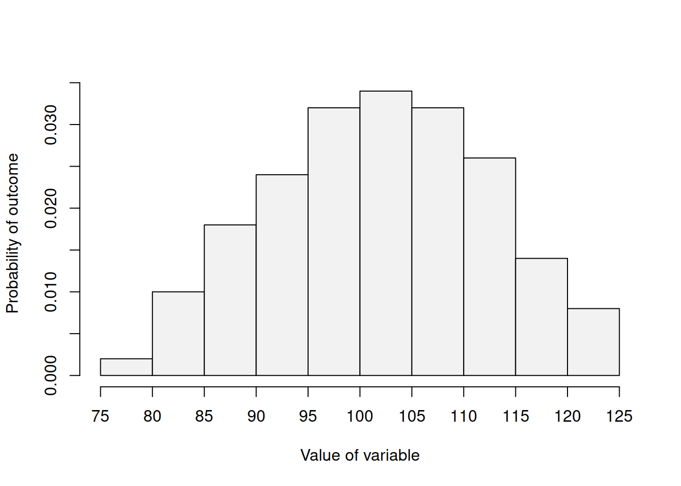
Figure 4.1: Distribution of a continuous random variable.
Based on Figure 4.1, we can say that the probability of obtaining the value between 100 and 105 is higher than for the variable to get any other interval. It also looks like the variable is continuous on the interval between 75 and 125, and we do not observe any values outside of this interval.
Almost any continuous distribution can be characterised by several functions:
- Probability density function (PDF);
- Cumulative distribution function (CDF);
- Quantile function (QF);
- Moment Generation Function (MMF);
- Characteristic function.
PDF has similarities with PMF, but does not return the probabilities, but rather the score for the variable in each specific point because (once again) the probability of continuous variable taking a specific value is equal to zero. PDF however is useful because it represents the shape of the distribution, showing where the values are concentrated. Figure 4.2 demonstrates an example of PDF of Normal distribution (discussed in more detail in Section 4.3).
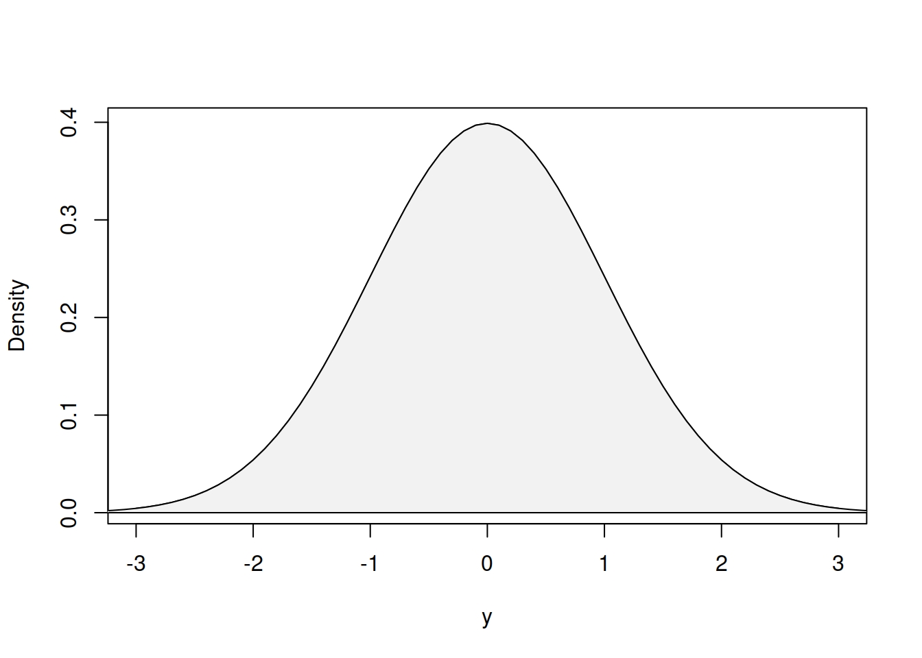
Figure 4.2: Probability Density Function of Normal distribution
It can be seen from the Figure 4.2 that the density of the distribution is higher at its centre, around zero, which means that it is more likely to get values around the centre rather than near the tails of the distribution.
If we want to work with probabilities in case of the continuous distribution, we need to use CDF, which is similar to the one discussed in the Chapter 3. Figure 4.3 shows example of CDF of Normal distribution.
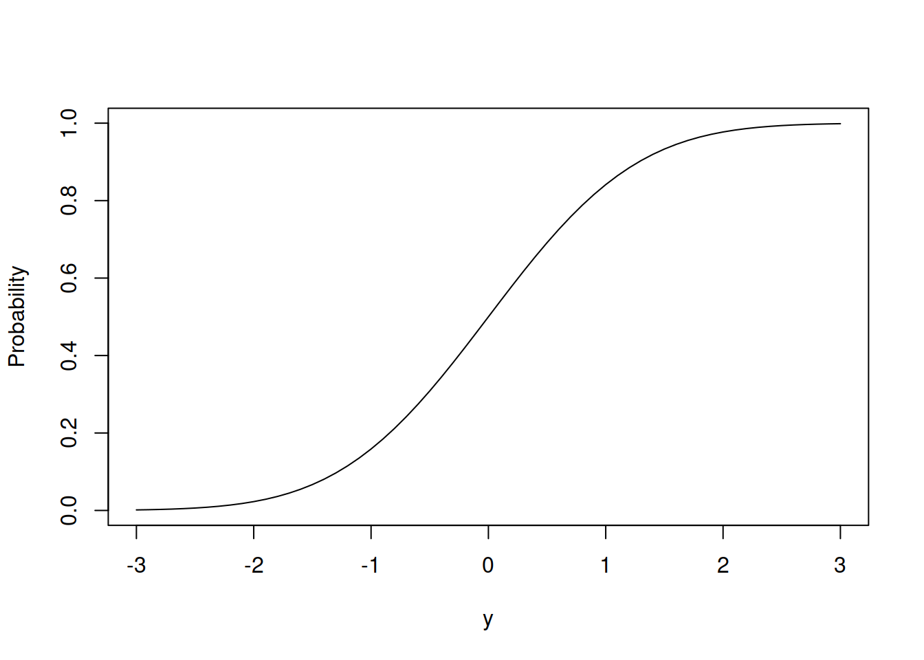
Figure 4.3: Cumulative Distribution Function of Normal distribution
The CDF of continuous variable has the same properties as CDF of the discrete one with the minor differences: in a general case it converges to one with the increase of the value \(y\) and converges to zero with the decrease of it. There are some continuous distributions that are restricted with an interval. For those distributions, the CDF reaches boundary values.
CDF is obtained by calculating the surface of PDF for each specific value of \(y\). Figure 4.4 shows the connection between them.
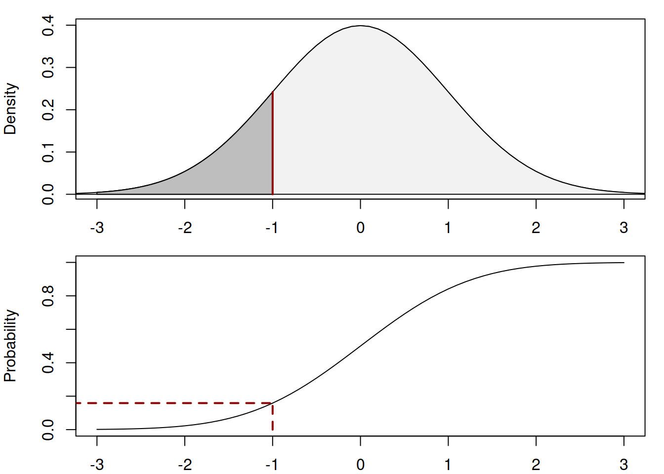
Figure 4.4: Cumulative Distribution Function of Normal distribution
The dark area in the first plot in Figure 4.4 is equal to the probability (the value on y-axis) in the second plot, which is approximately equal to 0.16.
Another important function is the Quantile Function. It returns the value of \(y\) for the given probability. By the definition, QF is the inverse of the CDF. It does not always have a closed form (thus cannot be represented mathematically), and for some distributions numerical optimisation is required to obtain the quantiles. Figure 4.5 demonstrates the quantile function of Normal distribution.
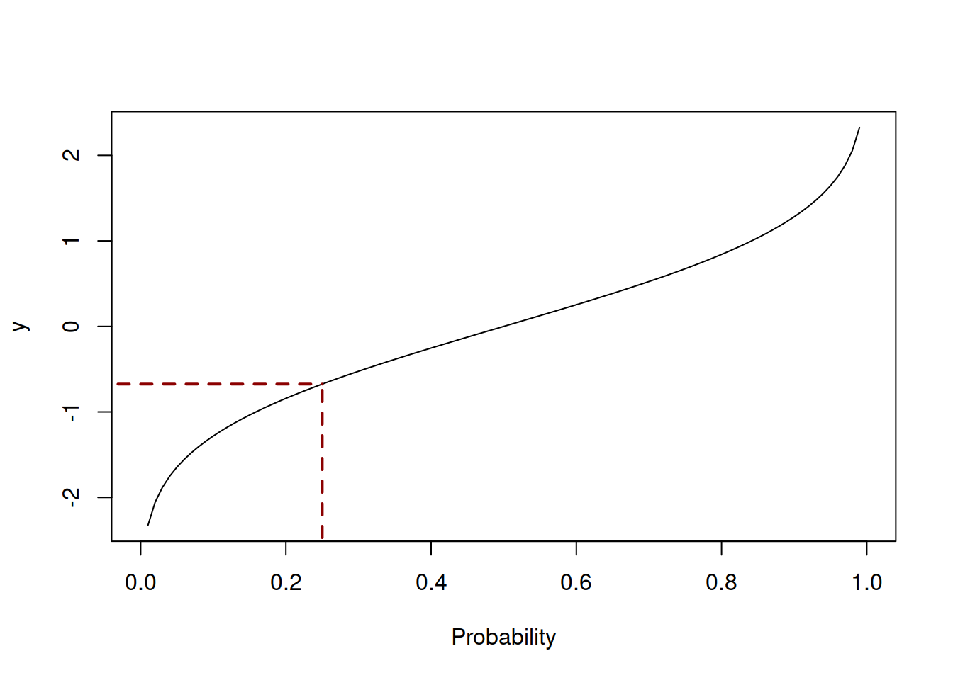
Figure 4.5: Quantile Function of Normal distribution
The dashed lines in Figure 4.5 show the value of \(y\) for the probability 0.25 according to the quantile function. In this example \(y \approx -0.68\), meaning that in 25% of the cases the random variable \(y\) will lie below this value. The quantiles of distributions are discussed in more detail in Section 5.1.
Finally, we have already mentioned MGF and CF in the context of discrete distributions. They play similar roles to the ones already discussed and can be used to obtain mean, variance, skewness and other statistics.