6.3 Central Limit Theorem
As we have already seen on Figure 6.3, the sample mean is not exactly equal to the population mean even when the sample size is very large (thousands of observations). There is always some sort of variability around the population mean. In order to understand how this variability looks like, we could conduct a simple experiment. We could take a random sample of, for instance, 1000 observations several times and record each of the obtained means. We then can see how the variable will be distributed to see if there are any patterns in the behaviour of the estimator (Figure 6.4):
obs <- 10000
# Set seed for reproducibility
set.seed(41)
# Define number of iterations
nIterations <- 1000
sampleSize <- 1000
# Generate data from normal distribution
y <- rnorm(obs,100,100)
yMean <- vector("numeric",nIterations)
for(i in 1:nIterations){
    yMean[i] <- mean(sample(y, sampleSize))
}
hist(yMean, xlab="Sample mean", main="", probability=TRUE,
     col=17)
# Add the density curve for the normal distribution
lines(seq(90,110,0.1),
      dnorm(seq(90,110,0.1), 100, 100/sqrt(sampleSize)),
      col=2, lwd=2)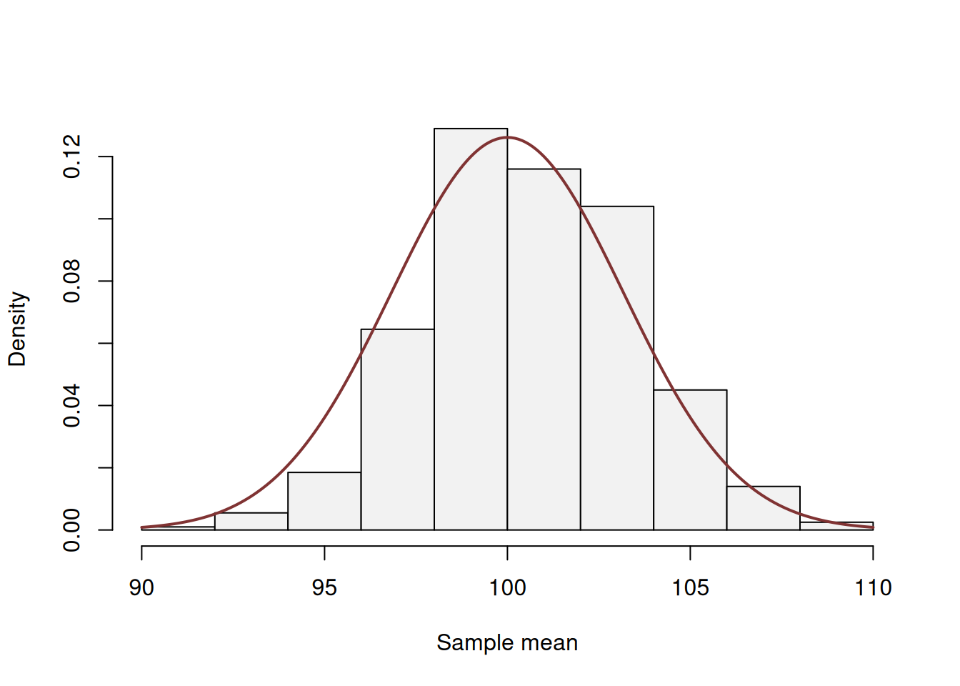
Figure 6.4: Histogram of the estimates of mean of the variable y.
Figure 6.4 shows the distribution of the estimates of mean and also has a density curve of the normal distribution with some known parameters above it. We can see that the empirical distribution on the histogram is pretty close to the normal one. In fact, to see this even clearer, we can produce a QQ-plot (discussed in Section 5.2) in Figure 6.5:
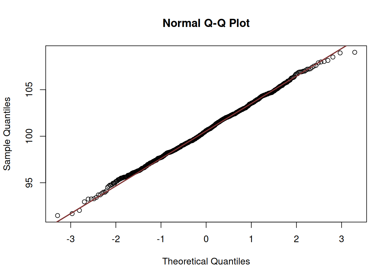
Figure 6.5: QQ-plot of the estimates of mean of the variable y.
We can see in Figure 6.5 that almost all points lie on the diagonal line, which indicates that the empirical quantiles are very close to the theoretical ones.
But why is that?
The answer to this is given by the so called “Central Limit Theorem”. It is a group of theorems proving that when many variables are added together, the distribution of their normalised sum asymptotically would follow the Normal distribution. There are many different versions of this theorem, which prove that it works under different conditions. One of the basic ones, tells that the sum of independent identically distributed random variables converges to the Normal distribution with the increase of the elements that are summed up, even if the distributions of each variable are not normal.
We do not prove the CLT here, but we provide a demonstration that explains how it holds. To do that, we need to refer back to the convolutions of distributions (Section 4.6). To understand why we refer to convolution, recall the formula for the sample mean: \[\begin{equation*} \bar{y} = \frac{1}{n} \sum_{j=1}^n y_j . \end{equation*}\] In the core of the calculation of the mean, there lies the sum of actual values \(y_j\). If each one of them has some distribution (e.g. Normal) then their mean would be the normalised (using \(n\)) sum of random variables \(y_j\).
Remark. The CLT is the theorem about what happens with the estimate (usually mean), not with individual observations. This means that the error term might follow, for example, Gamma distribution, but the estimate of its mean (under some conditions) will follow the Normal distribution.
Now, consider a simple case, where the random variable \(y\) follows the discrete Uniform distribution assuming values in the region [1, 6]. This corresponds to rolling a 6-sided die. If we now want to calculate the score of throwing several similar dice, we would be talking about the value \(z = y_1 + y_2 + y_3 + \dots + y_n = \sum_{j=1}^n y_j\), i.e. the convolution of \(n\) Uniform distributions. Figure 6.6 shows how the convolved distributions look for \(n=1\) (one die), \(n=2\) (two dice), \(n=4\) and \(n=8\).
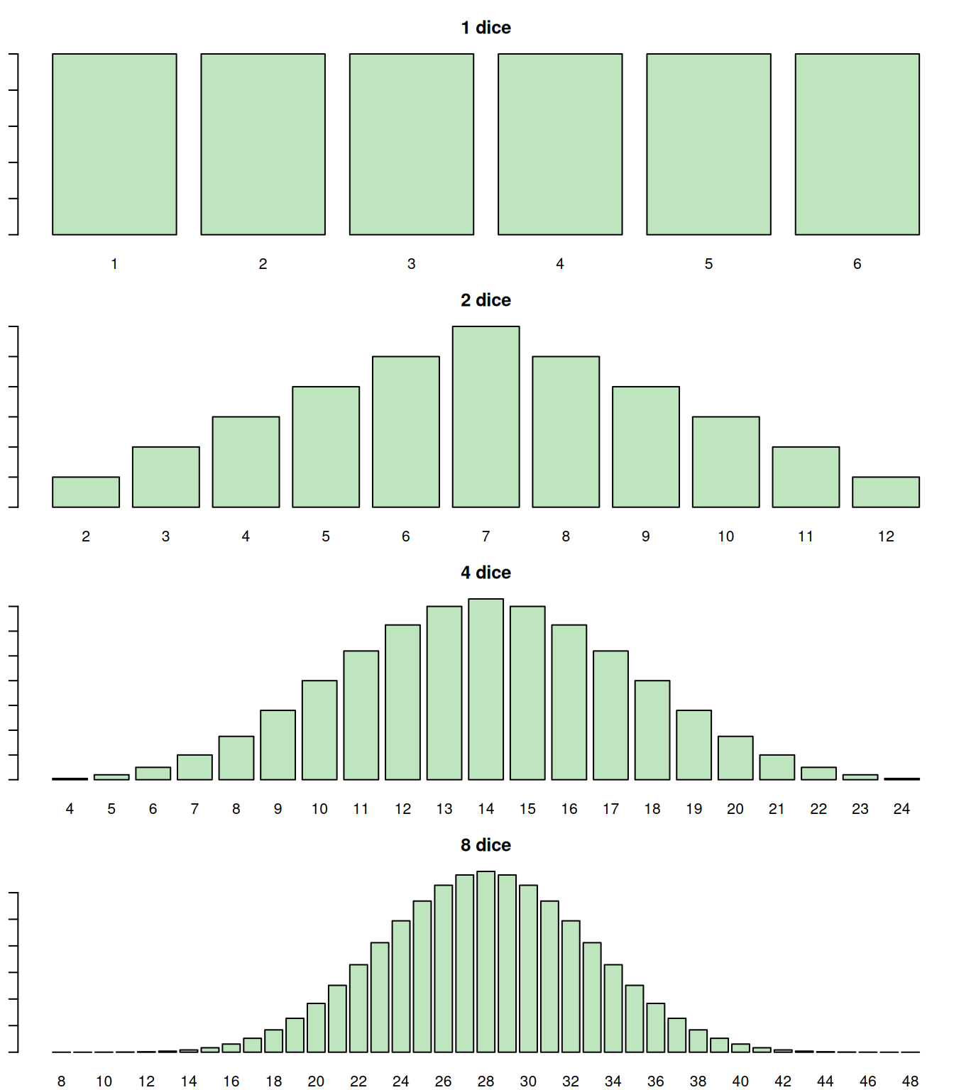
Figure 6.6: Probability Mass Function of the sum of n Uniform distributions for 1d6.
We see that the convolution of 8 distributions already starts looking similar to the normal one (Figure 6.6). The more dice we combine, the closer that distribution would be to the bell shape of the Normal distribution. This works for both discrete and continuous distributions, no matter what the original shape of the distribution is. The only thing that changes is the number of samples needed for the convolution to converge to the Normal one.
There are several factors that impact the speed of convergence of the convolution to the Normal distribution:
- Asymmetry of distribution - the more asymmetric the distribution of \(y\) is, the longer the sample size needs to be for the convolution to converge to the Normal distribution;
- Fatness of tails (or the sharpness of the peak) - the fatter the tails are, the longer the samples size needs to be for the convergence;
- Identical distribution - if all \(y_1\), \(y_2\), \(\dots\), \(y_n\) follow the same distribution, the speed of convergence will be higher;
- Independence of variables - if the variables are independent, the speed of convergence would be higher than in the case of dependent variables.
The fastest distribution, convolutions of which converge to the Normal one, is the Normal distribution itself. But even if the distribution of \(y_j\) is symmetric, without the large fat tails and the random variables \(y_j\) are i.i.d. (independent and identically distributed), then the speed of convergence would be high enough, so that even with the sample of 30 observations the empirical distribution of the sum \(\sum_{j=1}^n y_j\) would be close to the Normal one.
Now, consider several examples of distributions, violating the factors above. We will produce the empirical PDFs of the sum of \(n\) random variables and compared it with the Normal distribution.
Figure 6.7 demonstrates how probability density functions of the convolutions of the Log-Normal distributions would look, depending on how many variables \(y_j\) we sum up (for \(n=1, 2, 4, \dots 128\)). The distribution itself is asymmetric, which is apparent from the first image in Figure 6.7.
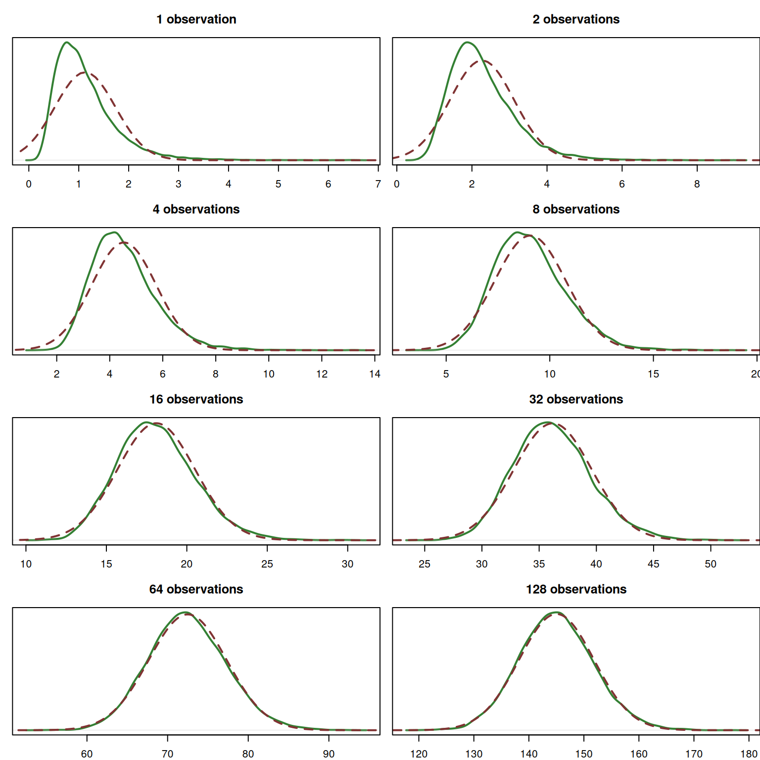
Figure 6.7: Probability Density Function of the convolution of n Log-Normal distributions, \(y \sim \mathrm{log}\mathcal{N}(0, 0.5)\).
The empirical density functions are shown in solid green line, while the normal distribution is shown in the dark red dashed lines. We can see that with the increase of the number of observations \(n\), the empirical density converges to the theoretical normal one. Given that the Log-Normal distribution is asymmetric, this convergence happens slowly, but even with the 64 samples, it looks already close to the Normal one.
Remark. The skewness of the Log-Normal distribution we considered in the example above is 1.7502. If the asymmetry of the distribution was higher, it would take more observations for the convolved distribution to converge to the Normal one.
Next, we see the effect of the fatness of tails. Figure 6.8 shows the convolution of the Laplace distributions. This distribution is known to have fatter tails and higher peak than the Normal one, which becomes apparent for the \(n=1\) in the figure.
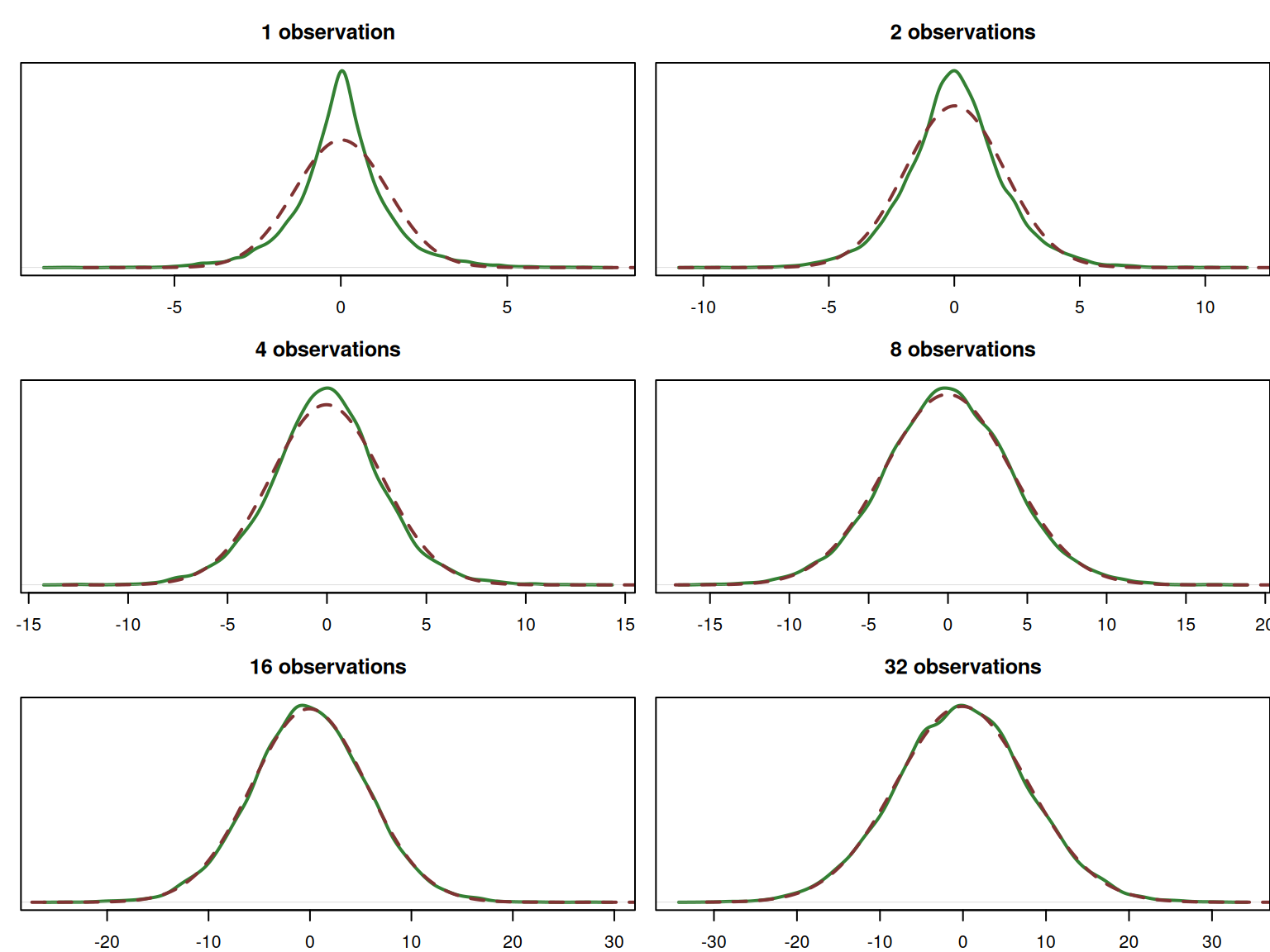
Figure 6.8: Probability Density Function of the sum of n Laplace distributions, \(y \sim \mathcal{Laplace}(0, 1)\).
But similarly to the example with the Log-Normal distribution, we see that the convolution of the Laplace distributions converges to the Normal one with the increase of the sample size. In fact, this happens much faster than in the case of the Log-Normal, and for the sample of 16 observations, the distributions already look very similar.
Remark. The excess kurtosis of the Laplace distribution is 3 (the Normal one has 0). In general, the higher it is for a distribution, the longer it will take (i.e. larger sample size) for the convolved distribution to converge to the Normal one.
Next, we consider the situation where the distributions are not identical. Figure 6.9 shows the convolution of several continuous distributions (with randomly selected parameters):
- Normal,
- Laplace,
- Log-Normal,
- Uniform,
- Gamma.
These are then normalised to have the same minimum and maximum values and are selected at random, after which their convolutions are plotted against the Normal density function.
Remark. While CLT works well for i.i.d. variables, for it to work in case of the violation of i.i.d., we need to normalise the random variables. Otherwise, some of them would dominate the pool and it would take many more samples for the convolved distribution to converge to the Normal one.
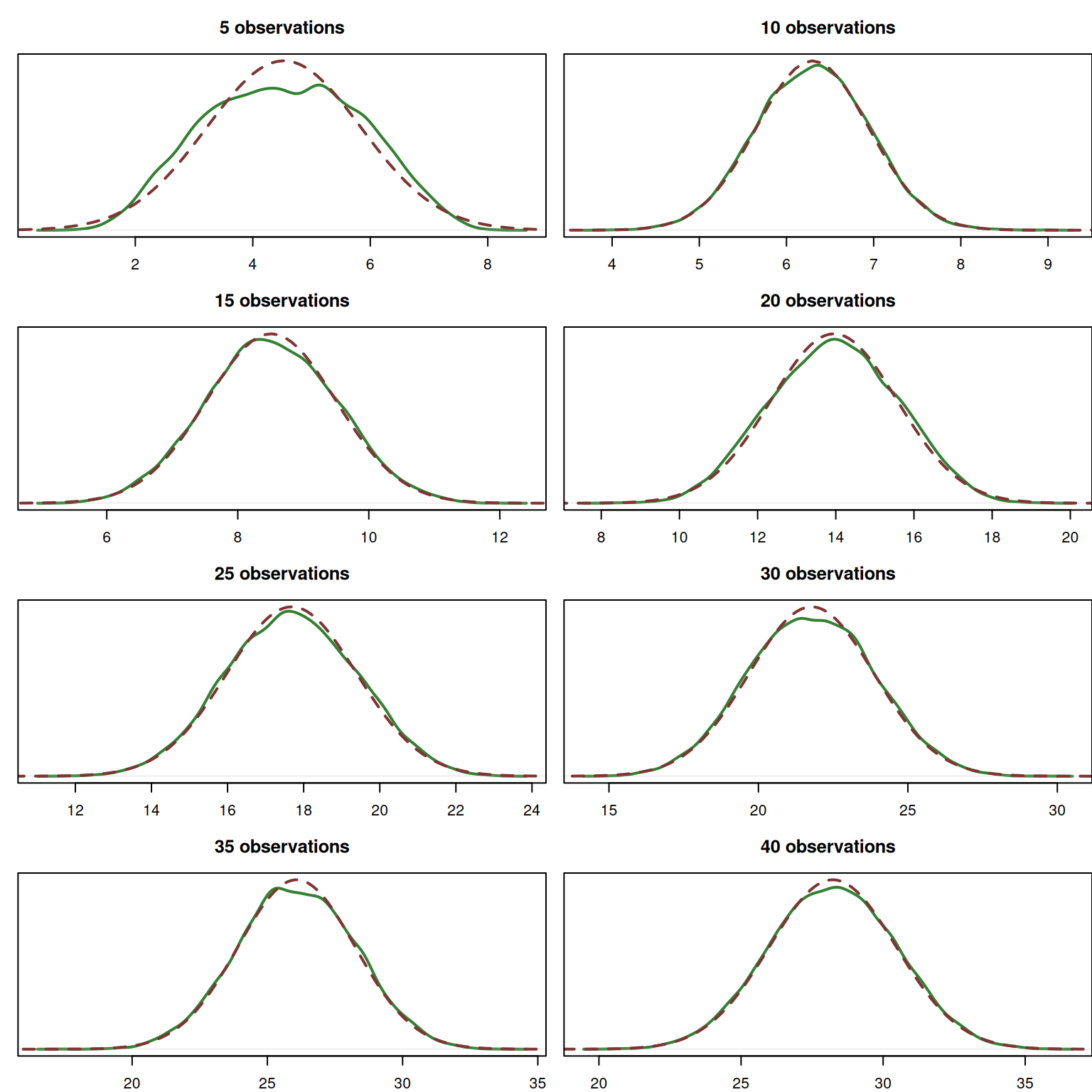
Figure 6.9: Probability Density Function of the sum of n non-identically distributed random variables.
As we see from Figure 6.9, the convolved distribution still converges to the Normal one, but this time the convergence happens non-linearly: adding asymmetric distributions to the pool leads to divergences from Normality on some of large samples (e.g. sample of 35 observations). But even in that case, the convolved distribution looks similar to the Normal one on larger samples.
The speed of convergence in this situation highly depends on the asymmetry and the excess of the convolved distributions (see two examples above).
Finally, we consider the violation of the independence. In this example, the variable \(y_j\) follows the normal distribution, but it’s parameters depend on the parameters of \(y_{j-1}\). Each value we generate is standardised to make sure that CLT works.
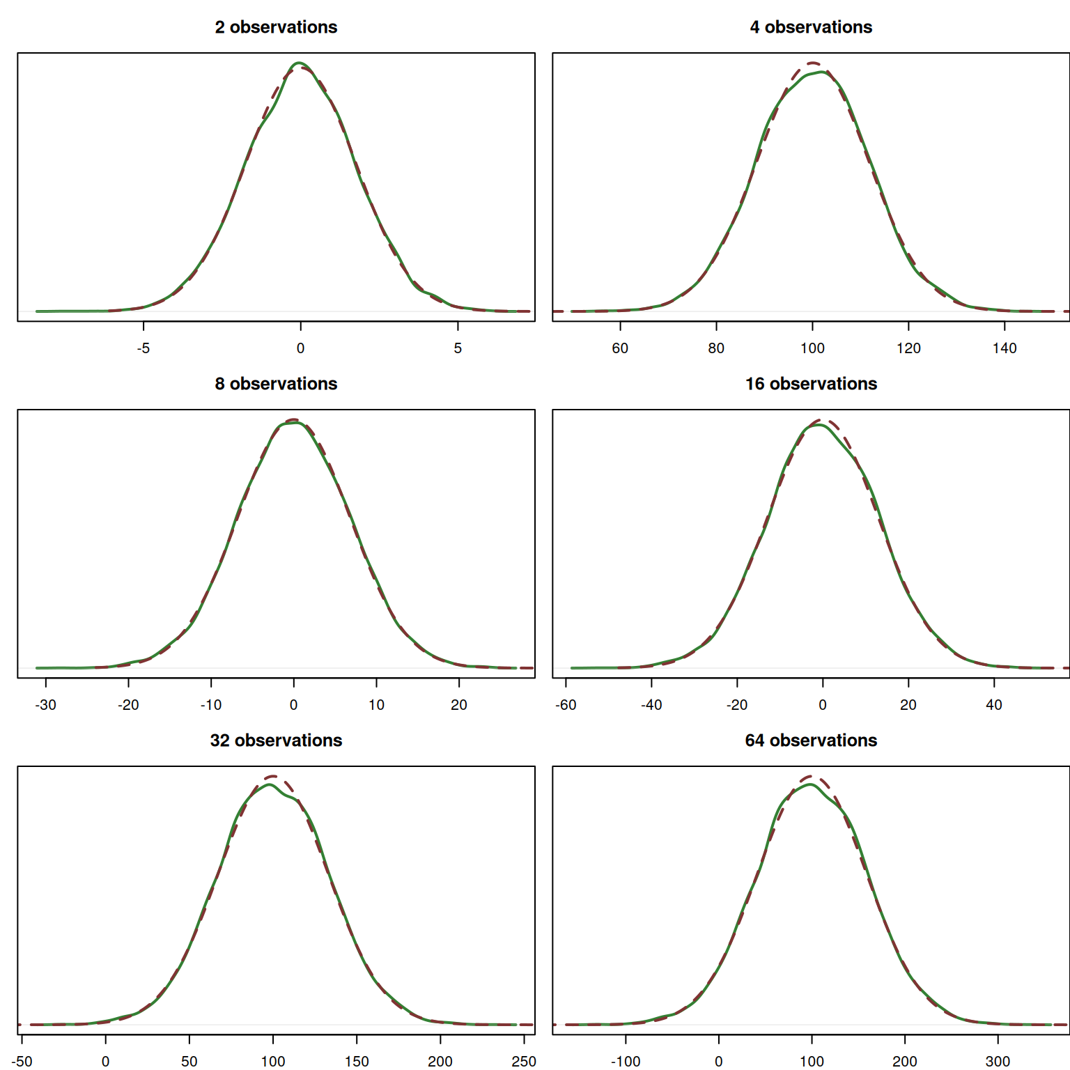
Figure 6.10: Probability Density Function of the sum of n dependent random variables.
Because the base distributions used in this example, are Normal, it does not take too much time for their convolution to get close to the Normal as well. Still, we see the violation of independence leads to shapes that deviate from normality even on the sample of 64 observations. The speed of convergence in this example would be lower if the convolved distributions are more linearly related.
In general, we should note that the more factors listed above are violated, the more observations you need to have before the Central Limit Theorem starts working and the convolved distribution becomes close to the Normal one. And as we saw from the examples above, the asymmetry is one of the critical factors influencing the speed of convergence of the convolution of distributions to the Normal one. But there are also three assumptions that need to be satisfied for the CLT to work at all:
- The true value of parameter is not near a bound. e.g. if the variable follows uniform distribution on (0, \(a\)) and we want to estimate \(a\), then its distribution will not be Normal (because in this case the true value is always approached from below). This assumption is important in contexts, where parameter estimates are restricted to make models obey some rules (e.g. AR parameters of ARIMA model that guarantee that it is stationary).
- The mean and variance of the distribution are finite. This might seem as a weird assumption, but some distributions do not have finite moments, so the CLT will not hold if a variable follows them, just because the sample mean will be all over the plane due to randomness and will not converge to the “true” value. Cauchy distribution is one of such examples.
- The random variables are independent identically distributed (i.i.d.). We saw what the violation of this assumption implies in milder cases, but in more serious ones, this might lead to more substantial problems, so that the convolved distribution would not converge to the Normal one.
If these assumptions hold, then CLT will work for the estimate of a parameter, no matter what the distribution of the random variable is. This becomes especially useful, when we want to test a hypothesis or construct a confidence interval for an estimate of a parameter.