10.4 Quality of a fit
The term “Quality of a fit” is used often in statistics to outline approaches that provide some information about how the applied models fit the data. We find it misleading, because the word “quality” is not appropriate here. The measures discussed in this section only show how well the actual values are approximated by the model, but their values do not tell us whether a model is good or bad. Still, to get a general impression about the performance of the estimated model, we can calculate several in-sample measures, which could provide us insights about the approximating properties of the model.
10.4.1 Sums of squares
The fundamental measure that lies in the basis of many other ones is SSE, which is the value of the OLS criterion (10.5). It cannot be interpreted on its own and cannot be used for model comparison, but it shows the overall variability of the data around the regression line. In a more general case, it is written as: \[\begin{equation} \mathrm{SSE} = \sum_{j=1}^n (y_j - \hat{y}_j)^2 . \tag{10.21} \end{equation}\] This sum of squares is related to another two, the first being the Sum of Squares Total: \[\begin{equation} \mathrm{SST}=\sum_{j=1}^n (y_j - \bar{y})^2, \tag{10.22} \end{equation}\] where \(\bar{y}\) is the in-sample mean. If we divide the value (10.22) by \(n-1\), we get the in-sample variance (introduced in Section 5.1): \[\begin{equation*} \mathrm{V}(y)=\frac{\mathrm{SST}}{n-1}=\frac{1}{n-1} \sum_{j=1}^n (y_j - \bar{y})^2 . \end{equation*}\] The last sum of squares is Sum of Squares of Regression: \[\begin{equation} \mathrm{SSR} = \sum_{j=1}^n (\bar{y} - \hat{y}_j)^2 , \tag{10.23} \end{equation}\] which shows the variability of the regression line. It is possible to show that in the linear regression (this is important, this property might be violated in other models), the three sums are related to each other via the following equation: \[\begin{equation} \mathrm{SST} = \mathrm{SSE} + \mathrm{SSR} . \tag{10.24} \end{equation}\]
Proof. This involves manipulations, some of which are not straightforward. First, we assume that SST equals to SSE + SSR, and see whether we reach the original formula of SST: \[\begin{equation} \begin{aligned} \mathrm{SST} &= \mathrm{SSR} + \mathrm{SSE} = \sum_{j=1}^n (\hat{y}_j - \bar{y})^2 + \sum_{j=1}^n (y_j - \hat{y}_j)^2 \\ &= \sum_{j=1}^n \left( \hat{y}_j^2 - 2 \hat{y}_j \bar{y} + \bar{y}^2 \right) + \sum_{j=1}^n \left( y_j^2 - 2 y_j \hat{y}_j + \hat{y}_j^2 \right) \\ &= \sum_{j=1}^n \left( \hat{y}_j^2 - 2 \hat{y}_j \bar{y} + \bar{y}^2 + y_j^2 - 2 y_j \hat{y}_j + \hat{y}_j^2 \right) \\ &= \sum_{j=1}^n \left(\bar{y}^2 -2 \bar{y} y_j + y_j^2 + 2 \bar{y} y_j + \hat{y}_j^2 - 2 \hat{y}_j \bar{y} - 2 y_j \hat{y}_j + \hat{y}_j^2 \right) \\ &= \sum_{j=1}^n \left((\bar{y} - y_j)^2 + 2 \bar{y} y_j + 2 \hat{y}_j^2 - 2 \hat{y}_j \bar{y} - 2 y_j \hat{y}_j \right) \end{aligned} . \tag{10.25} \end{equation}\] We can then substitute \(y_j=\hat{y}_j+e_j\) in the right hand side of (10.25) to get: \[\begin{equation} \begin{aligned} \mathrm{SST} &= \sum_{j=1}^n \left((\bar{y} - y_j)^2 + 2 \bar{y} (\hat{y}_j+e_j) + 2 \hat{y}_j^2 - 2 \hat{y}_j \bar{y} - 2 (\hat{y}_j+e_j) \hat{y}_j \right) \\ &= \sum_{j=1}^n \left((\bar{y} - y_j)^2 + 2 \bar{y} \hat{y}_j + 2 \bar{y} e_j + 2 \hat{y}_j^2 - 2 \hat{y}_j \bar{y} - 2 \hat{y}_j\hat{y}_j -2 e_j \hat{y}_j \right) \\ &= \sum_{j=1}^n \left((\bar{y} - y_j)^2 + 2 \bar{y} e_j + 2 \hat{y}_j^2 - 2 \hat{y}_j^2 -2 e_j \hat{y}_j \right) \\ &= \sum_{j=1}^n \left((\bar{y} - y_j)^2 + 2 \bar{y} e_j - 2 e_j \hat{y}_j \right) \end{aligned} . \tag{10.26} \end{equation}\] Now if we split the sum into three elements, we will get: \[\begin{equation} \begin{aligned} \mathrm{SST} &= \sum_{j=1}^n (\bar{y} - y_j)^2 + 2 \sum_{j=1}^n \left(\bar{y} e_j\right) - 2 \sum_{j=1}^n \left(e_j \hat{y}_j \right) \\ &= \sum_{j=1}^n (\bar{y} - y_j)^2 + 2 \bar{y} \sum_{j=1}^n e_j - 2 \sum_{j=1}^n \left(e_j \hat{y}_j \right) \end{aligned} . \tag{10.27} \end{equation}\] The second sum in (10.27) is equal to zero, because OLS guarantees that the in-sample mean of error term is equal to zero (see proof in Subsection 10.3). The third one can be expanded to: \[\begin{equation} \begin{aligned} \sum_{j=1}^n \left(e_j \hat{y}_j \right) = \sum_{j=1}^n \left(e_j b_0 + b_1 e_j x_j \right) \end{aligned} . \tag{10.28} \end{equation}\] We see the sum of errors in the first sum of (10.28), so the first elements is equal to zero again. The second term is equal to zero as well due to OLS estimation (this was also proven in Subsection 10.3). This means that: \[\begin{equation} \mathrm{SST} = \sum_{j=1}^n (\bar{y} - y_j)^2 , \tag{10.29} \end{equation}\] which is the formula of SST (10.22).
The relation between SSE, SSR and SST can be visualised and is shown in Figure 10.11. If we take any observation in that figure, we will see how the deviations from the regression line and from the mean are related.
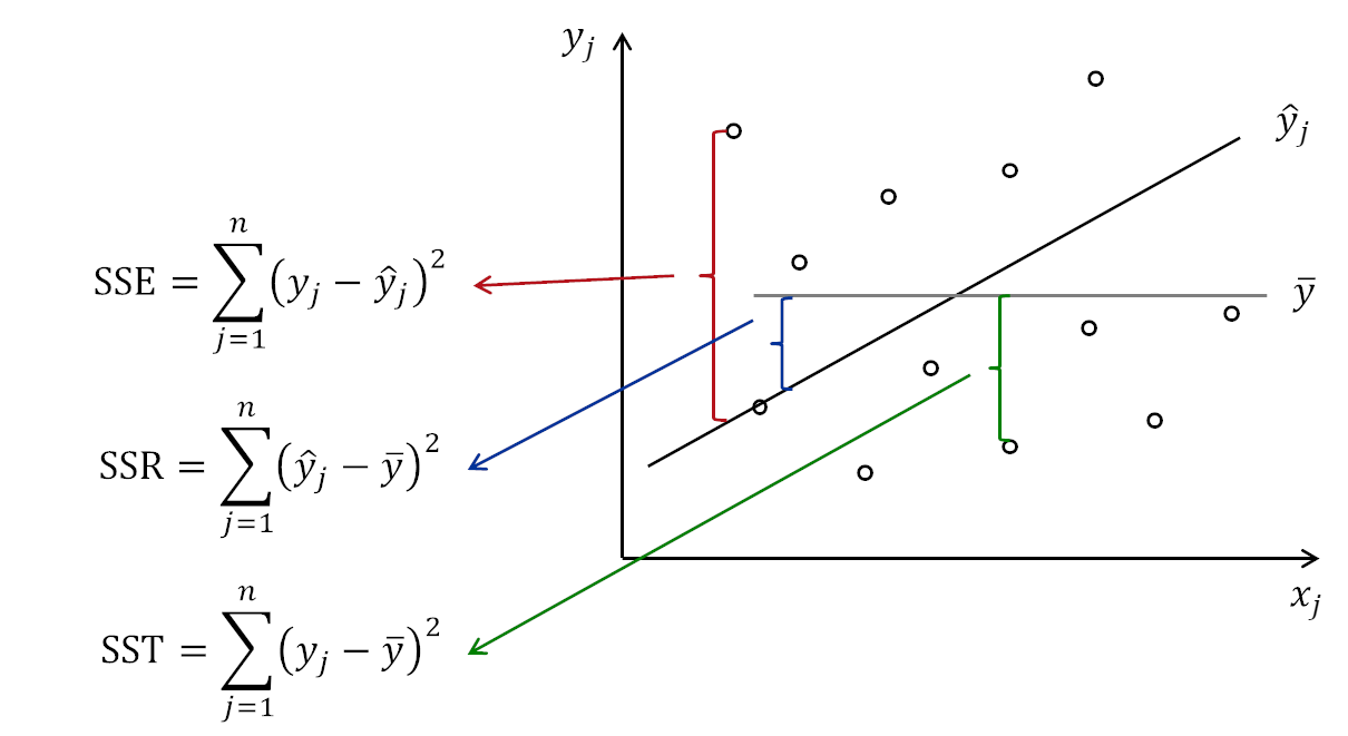
Figure 10.11: Relation between different sums of squares.
10.4.2 Coefficient of determination, R\(^2\)
While the sums of squares do not have a nice interpretation and are hard to use for diagnostics, they can be used in calculating the measure called “Coefficient of Determination”. It is calculated in the following way: \[\begin{equation} \mathrm{R}^2 = 1 - \frac{\mathrm{SSE}}{\mathrm{SST}} = \frac{\mathrm{SSR}}{\mathrm{SST}} . \tag{10.30} \end{equation}\] Given the fundamental property (10.24), we can see that R\(^2\) will always lie between zero and one. To better understand its meaning, imagine the following two extreme situations:
- The model fits the data in the same way as the mean line (black line coincides with the grey line in Figure 10.11). In this case SSE would be equal to SST and SSR would be equal to zero (because \(\hat{y}_j=\bar{y}\)) and as a result the R\(^2\) would be equal to zero.
- The model fits the data perfectly, without any errors (all points lie on the black line in Figure 10.11). In this situation SSE would be equal to zero and SSR would be equal to SST, because the regression would go through all points (i.e. \(\hat{y}_j=y_j\)). This would make R\(^2\) equal to one.
So, the zero value of the coefficient of determination means that the model does not explain the data at all and one means that it overfits the data. The value itself is usually interpreted as a percentage of variability in data explained by the model.
Remark. The properties above provide us an important point about the coefficient of determination: it should not be equal to one, and it is alarming if it is very close to one. This is because in this situation we are implying that there is no randomness in the data, which contradicts our definition of the statistical model (see Section 1.1.1). The adequate statistical model should always have some randomness in it. The situation of \(\mathrm{R}^2=1\) implies mathematically: \[\begin{equation*} y_j = b_0 + b_1 x_j , \end{equation*}\] which means that all \(e_j=0\), being unrealistic and only possible if there is a functional relation between \(y\) and \(x\) (no need for statistical inference then). So, in practice we should not maximise R\(^2\) and should be careful with models that have very high values of it. At the same time, too low values of R\(^2\) are also alarming, as they tell us that the model becomes: \[\begin{equation*} y_j = b_0 + e_j, \end{equation*}\] meaning that it is not different from the simple mean of the data, because in that case \(b_0=\bar{y}\). So, coefficient of determination in general is not a very good measure for assessing performance of a model. It can be used for further inferences, and for a basic indication of whether the model overfits (R\(^2\) close to 1) or underfits (R\(^2\) close to 0) the data. But no serious conclusions should be solely based on it.
Here how this measure can be calculated in R based on the model that we estimated in Section 10.1:
## [1] 0.357975Note that in this formula we used the relation between SST and V\((y)\), multiplying the value by \(n-1\) to get rid of the denominator. The resulting value tells us that the model has explained 35.8% deviations in the data.
Finally, based on coefficient of determination, we can also calculate the coefficient of multiple correlation, which we have already discussed in Section 9.4: \[\begin{equation} R = \sqrt{R^2} = \sqrt{\frac{\mathrm{SSR}}{\mathrm{SST}}} . \tag{10.31} \end{equation}\] It shows the closeness of relation between the response variable \(y_j\) and the explanatory variables to the linear one. The coefficient has a positive sign, no matter what the relation between the variables is. In case of the simple linear regression, it is equal to the correlation coefficient (from Section 9.3) with the sign equal to the sign of the coefficient of the slop \(b_1\) (this was discussed in Subsection 10.2.2): \[\begin{equation} r_{x,y} = \mathrm{sign} (b_1) R . \tag{10.32} \end{equation}\]
Here is a demonstration of the formula above in R:
##    height
## 0.5983101## [1] 0.5983101