15.2 Residuals are i.i.d.
There are five assumptions in this group:
- There is no autocorrelation in the residuals;
- The residuals are homoscedastic;
- The expectation of residuals is zero, no matter what;
- The variable follows the assumed distribution;
- More generally speaking, distribution of residuals does not change over time.
15.2.1 No autocorrelations
This assumption only applies to time series data, and in a way comes to capturing correctly the dynamic relations between variables. The term “autocorrelation” refers to the situation, when variable is correlated with itself from the past. If the residuals are autocorrelated, then something is neglected by the applied model. Typically, this leads to inefficient estimates of parameters, which in some cases might also become biased. The model with autocorrelated residuals might produce inaccurate point forecasts and prediction intervals of a wrong width (wider or narrower than needed).
There are several ways of diagnosing the problem, including visual analysis and statistical tests. In order to show some of them, we consider the Seatbelts data from datasets package for R. We fit a basic model, predicting monthly totals of car drivers in the Great Britain killed or seriously injured in car accidents:
In order to do graphical diagnose, we can produce plots of standardised / studentised residuals over time:
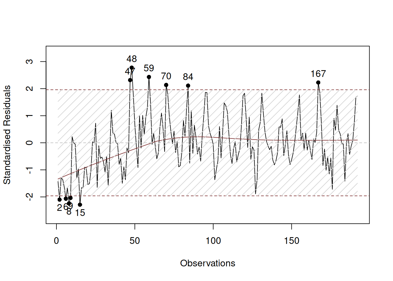
Figure 15.8: Standardised residuals over time.
If the assumption is not violated, then the plot in Figure 15.8 would not contain any patterns. However, we can see that, first, there is a seasonality in the residuals and second, the expectation (captured by the red LOWESS line) changes over time. This indicates that there might be some autocorrelation in residuals caused by omitted components. We do not aim to resolve the issue now, it is discussed in more detail in Section 14.5 of Svetunkov (2021).
The other instrument for diagnostics is ACF / PACF plots, which are produced in alm() via the following command:
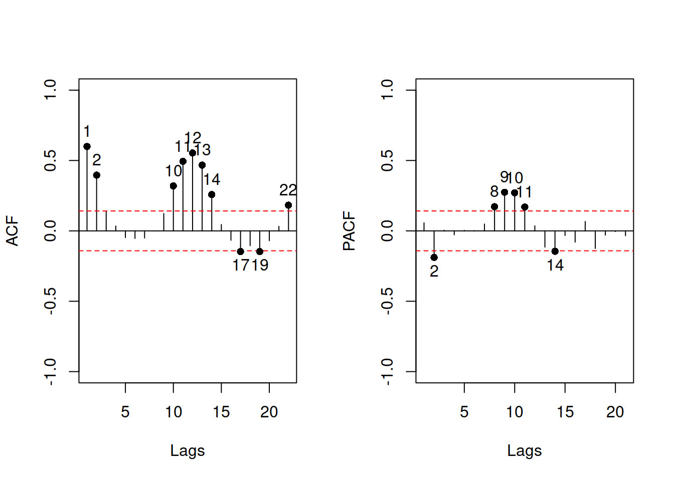
Figure 15.9: ACF and PACF of the residuals of a model.
15.2.2 Homoscedastic residuals
In general, we assume that the variance of residuals is constant. If this is violated, then we say that there is a heteroscedasticity in the model. This means that with a change of a variable, the variance of the residuals will change as well. If the model neglects this, then typically the estimates of parameters become inefficient and prediction intervals are wrong: they are wider than needed in some cases (e.g.m when the volume of data is low) and narrower than needed in the other ones (e.g. on high volume data).
Typically, this assumption will be violated if the model is not specified correctly. The classic example is the income versus expenditure on meals for different families. If the income is low, then there are not many options for buying, and the variability of expenses would be low. However, with the increase of income, the mean expenditures and their variability would increase because there are more options of what to buy, including both cheap and expensive products. If we constructed a basic linear model on such data, then it would violate the assumption of homoscedasticity and, as a result, will have issues discussed in section 15.2. But arguably, this would typically appear because of the misspecification of the model. For example, taking logarithms might resolve the issue in many cases, implying that the effect of one variable on the other should be multiplicative rather than additive. Alternatively, dividing variables by some other variable might (e.g. working with expenses per family member, not per family) resolve the problem as well. Unfortunately, the transformations are not the panacea, so in some cases, the analyst would need to construct a model, taking the changing variance into account (e.g. GARCH or GAMLSS models). This is discussed in Section ??.
While forecasting, we are more interested in the holdout performance of models, in econometrics, the parameters of models are typical of the main interest. And, as we discussed earlier, in the case of a correctly specified model with heteroscedastic residuals, the estimates of parameters will be unbiased but inefficient. So, econometricians would use different approaches to diminish the heteroscedasticity effect on parameters: either a different estimator for a model (such as Weighted Least Squares) or a different method for calculating standard errors of parameters (e.g. Heteroskedasticity-Consistent Standard Errors). This does not resolve the problem but instead corrects the model’s parameters (i.e. does not heal the illness but treats the symptoms). Although these approaches typically suffice for analytical purposes, they do not fix the issues in forecasting.
The diagnostics of heteroscedasticity can be done via plotting absolute and / or squared residuals against the fitted values.
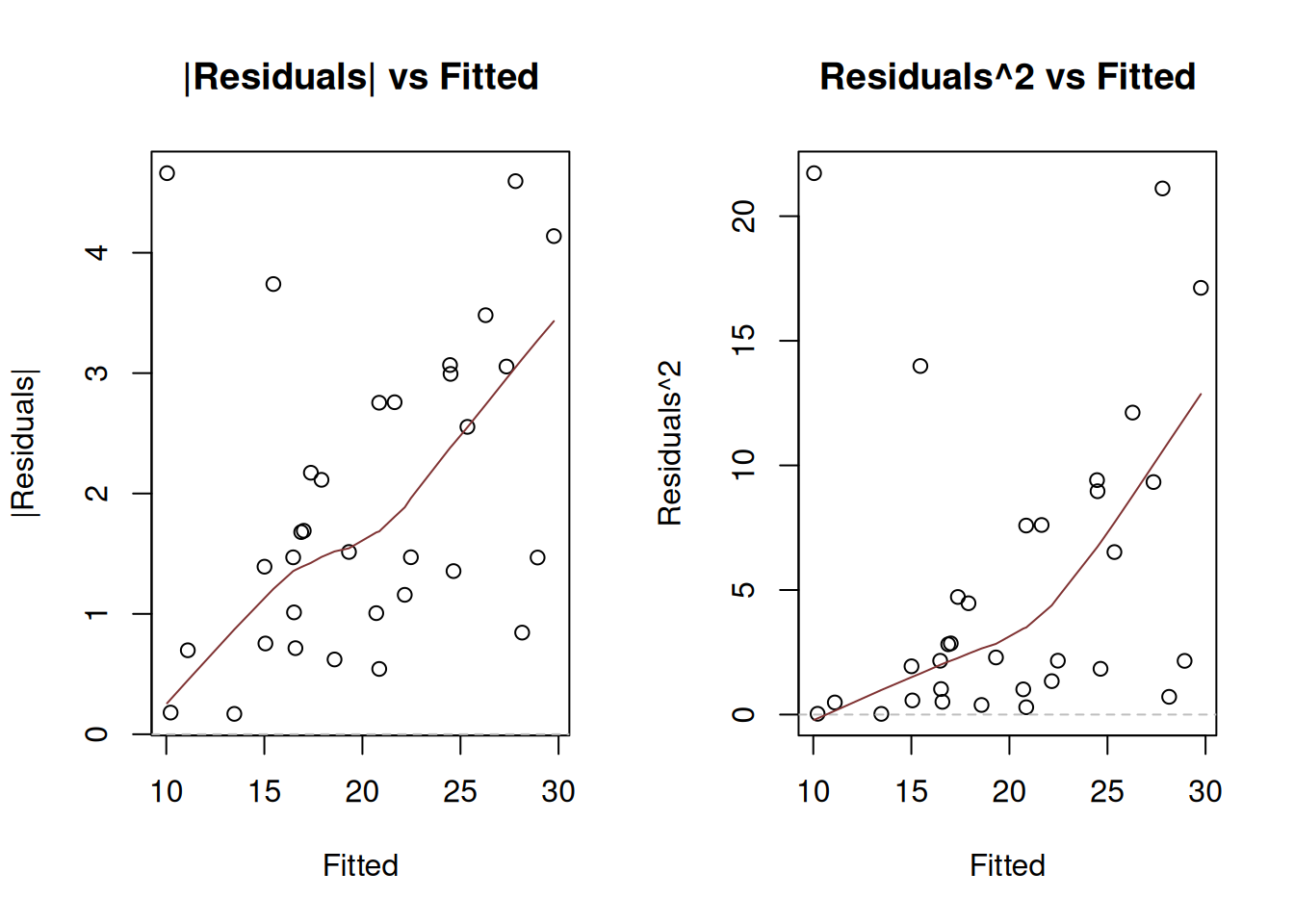
Figure 15.10: Detecting heteroscedasticity. Model 1.
If your model assumes that residuals follow a distribution related to the Normal one, then you should focus on the plot of squared residuals vs fitted, as this would be closer related to the variance of the distribution. In the example of mtcars model in Figure 15.10 we see that the variance of residuals increases with the increase of Fitted values (the LOWESS line increases and the overall variability around 1200 is lower than the one around 2000). This indicates that the residuals are heteroscedastic. One of the possible solutions of the problem is taking the logarithms, as we have done in the model mtcarsALM02:
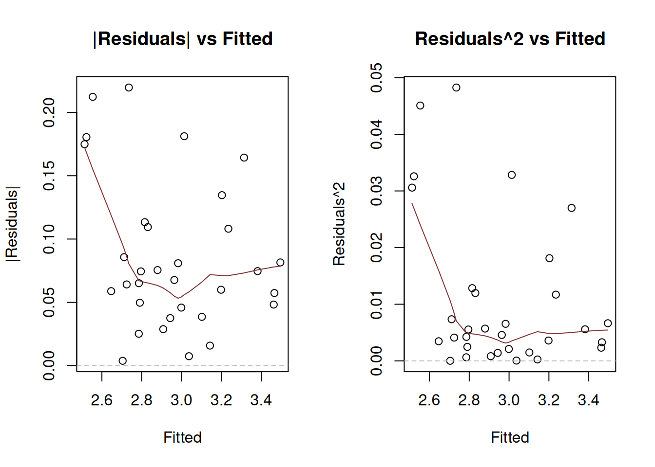
Figure 15.11: Detecting heteroscedasticity. Model 2.
While the LOWESS lines on plots in Figure 15.11 demonstrate some dynamics, the variability of residuals does not change significantly with the increase of fitted value, so non-linear transformation seems to fix the issue in our example. If it would not, then we would need to consider either some other transformations or finding out, which of the variables causes heteroscedasticity and then modelling it explicitly via the scale model (Section ??).
15.2.3 Mean of residuals
While in sample, this holds automatically in many cases (e.g. when using Least Squares method for regression model estimation), this assumption might be violated in the holdout sample. In this case the point forecasts would be biased, because they typically do not take the non-zero mean of forecast error into account, and the prediction interval might be off as well, because of the wrong estimation of the scale of distribution (e.g. variance is higher than needed). This assumption also implies that the expectation of residuals is zero even conditional on the explanatory variables in the model. If it is not, then this might mean that there is still some important information omitted in the applied model. This implies that the following holds for all \(x_i\): \[\begin{equation*} \mathrm{cov}(x_i, e) = 0 , \end{equation*}\] which in the case of \(\mathrm{E}(e)=0\) is equivalent to: \[\begin{equation*} \mathrm{E}(x_i e) = 0 . \end{equation*}\] If OLS is used in linear model estimation, then this condition is satisfied in sample automatically and does not require checking.
Note that some models assume that the expectation of residuals is equal to one instead of zero (e.g. multiplicative error models). The idea of the assumption stays the same, it is only the value that changes.
The diagnostics of the problem would be similar to the case of non-linear transformations or autocorrelations: plotting residuals vs fitted or residuals vs time and trying to find patterns. If the mean of residuals changes either with the change of fitted values of with time, then the conditional expectation of residuals is not zero, and something is missing in the model.
15.2.4 Distributional assumptions
In some cases we are interested in using methods that imply specific distributional assumptions about the model and its residuals. For example, it is assumed in the classical linear model that the error term follows Normal distribution. Estimating this model using MLE with the probability density function of Normal distribution or via minimisation of Mean Squared Error (MSE) would give efficient and consistent estimates of parameters. If the assumption of normality does not hold, then the estimates might be inefficient and in some cases inconsistent. When it comes to forecasting, the main issue in the wrong distributional assumption appears, when prediction intervals are needed: they might rely on a wrong distribution and be narrower or wider than needed. Finally, if we deal with the wrong distribution, then the model selection mechanism might be flawed and would lead to the selection of an inappropriate model.
The most efficient way of diagnosing this, is constructing QQ-plot of residuals (discussed in Section 5.2).
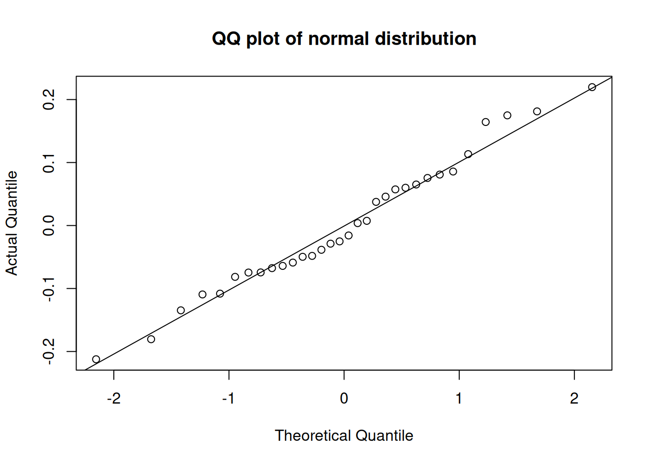
Figure 15.12: QQ-plot of residuals of model 2 for mtcars dataset.
Figure 15.12 shows that all the points lie close to the line (with minor fluctuations around it), so we can conclude that the residuals follow the normal distribution. In comparison, Figure 15.12 demonstrates how residuals would look in case of a wrong distribution. Although the values lie not too far from ths straight line, there are several observations in the tails that are further away than needed. Comparing the two plots, we would select the on in Figure 15.12, as the residuals are better behaved.
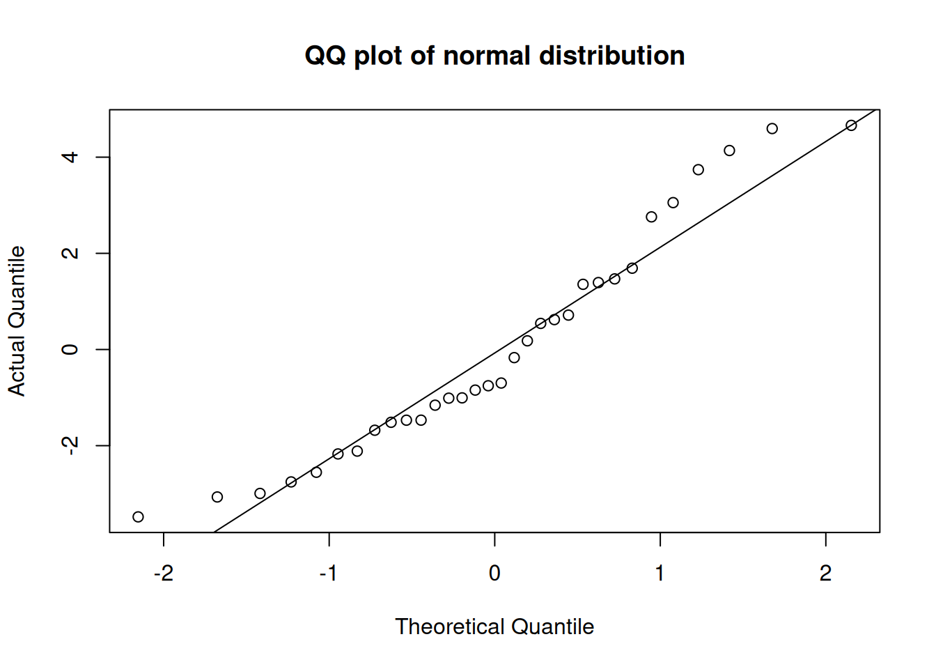
Figure 15.13: QQ-plot of residuals of model 1 for mtcars dataset.
15.2.5 Distribution does not change
This assumption aligns with the Subsection 15.2.4, but in this specific context implies that all the parameters of distribution stay the same and the shape of distribution does not change. If the former is violated then we might have one of the issues discussed above. If the latter is violated then we might produce biased forecasts and underestimate / overestimate the uncertainty about the future. The diagnosis of this comes to analysing QQ-plots, similar to Subsection 15.2.4.