6.2 Law of Large Numbers
Coming back to the example with the height of students, what we might notice in such experiment that with the increase of the sample size, the average height would tend to slowly converge to some value. This is captured by one of the fundamental laws of statistics, called the Law of Large Numbers (LLN). It is the theorem saying that (under wide conditions) the average of a variable obtained over the large number of trials will be close to its expected value and will get closer to it with the increase of the sample size. This can be demonstrated with the following artificial example:
obs <- 10000
set.seed(42)
# Generate data from normal distribution
y <- rnorm(obs,100,50)
# Create sub-samples of 30 and 1000 observations
y30 <- sample(y, 30)
y1000 <- sample(y, 1000)
par(mfcol=c(1,2))
hist(y30, xlab="y", col=17,
     main="Sample of 30", xlim=c(-100,300))
abline(v=mean(y30), col=2, lwd=2)
hist(y1000, xlab="y", col=17,
     main="Sample of 1000", xlim=c(-100,300))
abline(v=mean(y1000), col=2, lwd=2)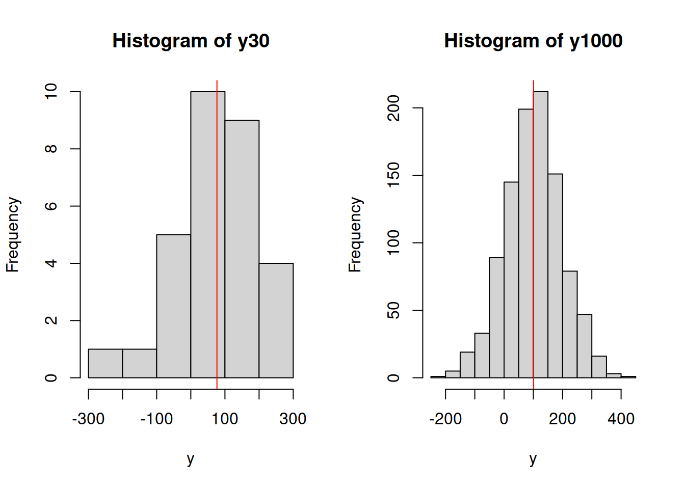
Figure 6.2: Histograms of samples of data from variable y.
What we can see on the plots in Figure 6.2 is that the mean (red vertical line) on the left plot will be further away from the true mean of 100 than in the case of the right one. Given that this data is randomly generated, the situation might differ, but the idea would be that with the increase of the sample size the estimated sample mean will converge to the true one. We can even produce a plot showing how this happens:
yMeanLLN <- vector("numeric",obs)
set.seed(42)
for(i in 1:obs){
    yMeanLLN[i] <- mean(sample(y,i))
}
plot(yMeanLLN, type="l", xlab="Sample size", ylab="Sample mean")
abline(h=100, col=5, lty=2)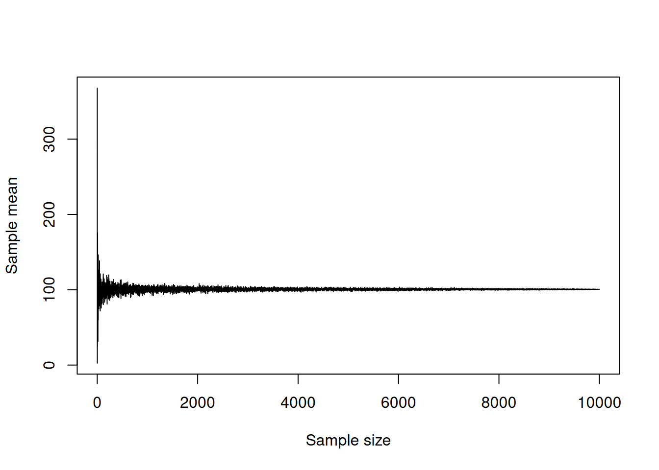
Figure 6.3: Demonstration of Law of Large Numbers.
We can see from the plot above that with the increase of the sample size the sample mean gets closer to the true value of 100. This is a graphical demonstration of the Law of Large Numbers: it only tells us what will happen when the sample size increases and becomes large enough. But it is still useful, because it demonstrates the “gravity” of sampling, and if it does not work, then the estimate of the mean would be incorrect. In that case, we would not be able to make conclusions about the behaviour in population.
In order for LLN to work, the distribution of variable needs to have finite mean and variance. This is discussed in some detail in Section 6.3.
In summary, what LLN tells us is that if we average things out over a large number of observations, then that average starts looking very similar to the population value. However, this does not say anything about the performance of estimators on small samples.