3.7 Negative Binomial distribution
One of the tasks in manufacturing is to understand how many days it might take for a machine to break. In this case, everyday when it works we could encode as a “failure to break”, and when it breaks, we would encode it as “success”. Assuming that there are many small unpredictable factors impacting the possibility to break, we can safely assume that there is a fixed probability that this will happen. Can we somehow model this process to make adequate decisions about the work of the machine?
Yes. The Negative Binomial distribution is one of the appropriate tools here. It models the number of failures in an experiment (no breaks in our example) before some defined number of successes occurs. In contrast with the Binomial distribution, in the NegBin, the number of the total trials is unknown. And in the example above, we could say that a success is when the machine stops working.
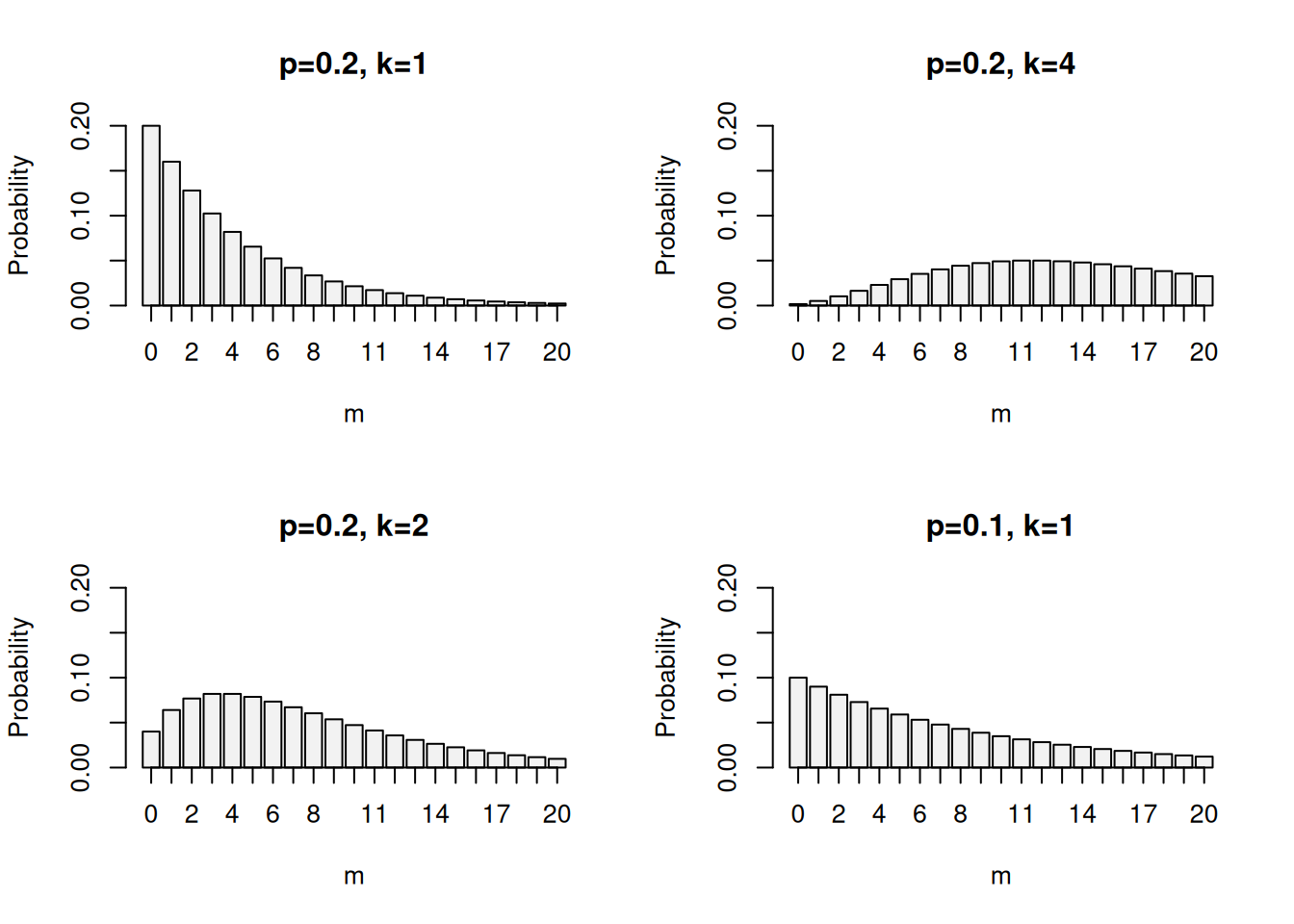
Visually, the PMF of the NegBin can be represented in the following way (Figure 3.11) with \(p\) being the probability of success, \(k\) being the number of successes before the experiment stops, and \(m\) being the number of failures.

Figure 3.11: PMF of the Negative Binomial distribution with different probabilities and number of successes \(k\).
Figure 3.11 shows that, for example, if p=0.2, and we want to have one success (k=1), we have the probability of 0.2 that we will succeed without having any failures. To make this easier to understand, if we have a 1d5 (five-sided dice), and we define success as rolling 5 on it, the probability that we will have it in the first roll is 0.2 (this is one out of five possible outcomes), which corresponds to the first bar in the first plot in Figure 3.11. The probability that we will roll 5 in the second trial is \(0.2 \times (1-0.2) = 0.16\), which corresponds to the second bar in the first plot in Figure 3.11, and so on. With \(k=2\), a situation is modelled when we need to get five on a dice two times in an experiment (not necessarily sequentially). The calculation of the specific probability becomes more complicated with the incrase of \(k\). But in general, the PMF of the Negative Binomial distribution is written as: \[\begin{equation} f(m, k, p) = \begin{pmatrix} k+m-1 \\ m \end{pmatrix} p^k (1-p)^m , \tag{3.19} \end{equation}\] where \(k\) is the number of successes and \(m\) is the number of failures. This PMF is very similar to the one of the Binomial distribution, but it is parametrised differently, which makes it useful in some contexts (like the one mentioned in the beginning of this section).
The characteristics of the Negative Binomial distribution are similar to the Binomial one, discussed in Section 3.4, except for the last (fifth) element: the number of overall trials in the NegBin is unknown.
The mean and standard deviations of the distribution are defined as: \[\begin{equation} \mathrm{E}(y) = k \frac{1-p}{p} \tag{3.20} \end{equation}\] and \[\begin{equation} \mathrm{V}(y) = k \frac{1-p}{p^2} \tag{3.21} \end{equation}\] respectively.
We do not provide the formula for the CDF here, because it is quite complicated.
A machine in a factory works only when at least one of the three independent components works. The probability of a break of each component is estimated to be 0.1. How many days would it take on average for the machine to stop working? What is the probability that the machine will work exactly for a month (30 days)?
Solution. In this task, we use the Negative Binomial distribution because:
- There are many potential trials;
- In each trial, there are only two outcomes: components work or fail;
- The probability of success (a component breaks) is fixed between the trials;
- The trials are independent: if one component fails, this should not impact the work of the other one;
- The number of trials \(n\) is unknown.
The probability of failure (success in the terms of NegBin) is \(p=0.1\). The number of components, \(k=3\). This is all we need to know to use the distribution and answer the questions.
The average number of days until the machine stops working is calculated using (3.20): \[\begin{equation} \mathrm{E}(y) = 3 \frac{1-0.1}{0.1} = 27 \tag{3.20} \end{equation}\] As for the answer to the second question, working for exactly 30 days means that the machine will break on the 31st day. We can use the PMF, specifying \(m=30\): \[\begin{equation*} f(30, 3, 0.1) = \begin{pmatrix} 30+3-1 \\ 3 \end{pmatrix} 0.1^3 (1-0.1)^30 \approx 0.021 . \end{equation*}\]
In R, the Negative Binomial distribution is implemented in the functions rnbinom(), dnbinom(), pnbinom(), and qnbinom(), implementing the random function, the PMF, the CDF and the QF respectively. Here how the PMF can be used to get the answer to the question in the previous task:
## [1] 0.02102601