3.3 Bernoulli distribution (Tossing a coin)
Consider a case when we track whether it rains at Lancaster or not and want to understand based on this information whether it will rain today or not. In this example, we have two values for a random variable (1 - it rains, 0 - it does not), and if we do not have any additional information, we assume that the probability that it rains is fixed. This situation can be modelled using the Bernoulli distribution.
It is one of the simplest distributions. It can be used to characterise the situation, when there are only two outcomes of event, like the classical example with coin tossing. In this special case, according to this distribution, the random variable can only take two values: zero (e.g. for heads) and one (e.g. tails) with a probability of having tails equal to \(p=0.5\). It is a useful distribution not only for the coin experiment, but for any other experiment with two outcomes and some probability \(p\). For example, consumers behaviour when making a choice whether to buy a product or not can be modelled using Bernoulli distribution: we do not know what a consumer will choose and why, so based on some external information we can assign them a probability of purchase \(p\).
In general, the distribution can be characterised with the following PMF: \[\begin{equation} f(y, p) = p^y (1-p)^{1-y}, \tag{3.3} \end{equation}\] where \(y\) can only take values of 0 and 1. Figure 3.3 demonstrates how the PMF (3.3) looks for several probabilities.
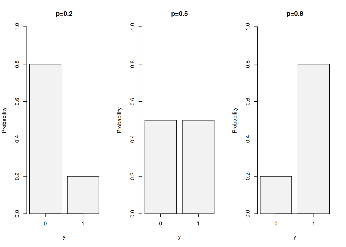
Figure 3.3: Probability Mass Function of Bernoulli distribution with probabilities of 0.2, 0.5 and 0.8
The mean of this distribution equals to \(p\), which is in practice used in the estimation of the probability of occurrence \(p\): collecting a vector of zeroes and ones and then taking the mean will give the empirical probability of occurrence \(\hat{p}\). The variance of Bernoulli distribution is \(p\times (1-p)\).
Finally, the CDF of the distribution is: \[\begin{equation} F(y, p) = \left\{ \begin{aligned} 1-p, & \text{ for } y=0 \\ 1, & \text{ for } y=1 . \end{aligned} \right. \tag{3.4} \end{equation}\] which can be plotted as shown in Figure 3.4.
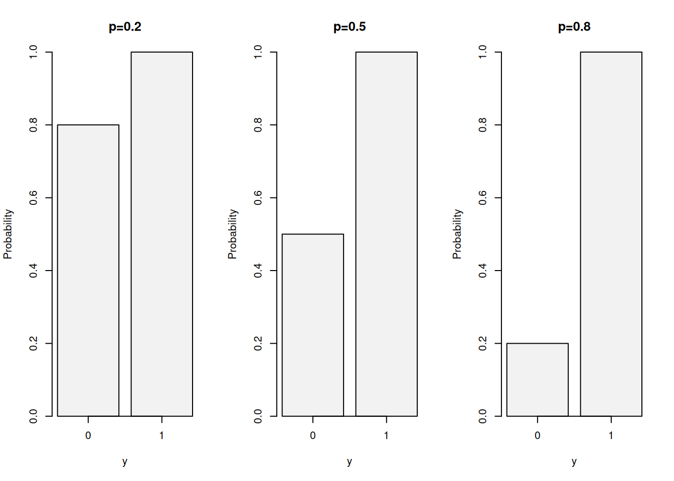
Figure 3.4: Cumulative Distribution Function of Bernoulli distribution with probabilities of 0.2, 0.5 and 0.8
The CDF of Bernoulli distribution is seldom used in practice and is provided here for completeness.
While sitting at home during the COVID pandemic isolation, Vasiliy conducted an experiment: he threw paper balls in a rubbish bin located in the far corner of his room. He counted how many times he missed and how many times he got the balls in the bin. It was 36 to 64.
- What is the probability distribution that describes this experiment?
- What is the probability that Vasiliy will miss when he throws the next ball?
- What is the variance of his throws?
Solution. This is an example of Bernoulli distribution: it has two outcomes and a probability of success.
We will encode the miss as zero and the score as one. Based on that, taking the mean of the outcomes, we can estimate the mean of Bernoulli probability of miss: \[\begin{equation*} \bar{y} = \hat{p} = \frac{36}{100} = 0.36. \end{equation*}\] So, when Vasiliy throws the next ball in the bin, he will miss with the probability of 0.36.
The variance is \(p \times (1-p) = 0.36 \times 0.64 = 0.2304\).
In R, this distribution is implemented in stats package via dbinom(size=1), pbinom(size=1), qbinom(size=1) and rbinom(size=1) for PDF, CDF, QF and random generator respectively. The important parameter in this case is size=1, which will be discussed in Section 3.4.
Remark. A nice example of a task using Bernoulli distribution is the Saint Petersburg Paradox (Kotz et al., 2005, p. 8318). The idea of it is as follows. Imagine that I offer you to play a game. I will toss the coin as many times as needed to get first heads. We will calculate how many tails I had in that tossing and I will pay you an amount of money, depending on that number. If I toss tails once, I will pay you £2. If I toss it twice, I will pay £\(2^2=4\). In general, I will pay £\(2^n\) if I toss consecutively \(n\) tails before getting heads. The question of this task, is how much you will be ready to pay to enter such game (i.e. what is the fair price?). Daniel Bernoulli proposed that the fair price can be calculated via the expectation of prize, which in this case is: \[\begin{equation*} \mathrm{E}(\text{tails }n\text{ times and heads on }n+1) = \sum_{j=1}^\infty 2^{j} \left(\frac{1}{2}\right)^{j+1} \end{equation*}\] The logic behind this formula is that mathematically, we assume that we can have infinite number of experiments, and each prize has its outcome. For example, the probability to get just £2 is \(\frac{1}{2}\), while the probability to get £4 is \(\frac{1}{4}\) etc. But the values cancel each other out in this formula leaving us with: \[\begin{equation*} \mathrm{E}(\text{tails }n\text{ times and heads on }n+1) = \sum_{j=1}^\infty \frac{1}{2} = \infty . \end{equation*}\] So, although it is unrealistic to expect in real life that the streak of tails will continue indefinitely, the statistics theory tells us that the fair price for the game is infinity. Practically speaking, the infinite amount of tails will never happen, so we should have a finite number for the price. But mathematics assumes that the experiment can be repeated infinite amount of times, and in this case it is entirely possible that we will observe an infinite streak of tails. This is the Saint Petersburg paradox, which demonstrates how sometimes the asymptotic properties relate to reality. I think that it provides a good demonstration of what statistics typically works with.
Finally, coming back to the rain example, we cannot say for sure whether it will rain tomorrow or not, but based on the collected sample, we can calculate the probability of that event. But remember that even if the probability is low, it does not mean that you do not need to bring an umbrella with you.