7.3 Power of a test
Consider a situation when we want to know average income of people living in a country across two regions, and we want to find out whether those averages are similar or not. We could ask “what’s your yearly income” for ten people in each of the regions, calculate means and compare them using some statistical test (these will be discussed in Chapter 8). If the average incomes are in reality indeed different, we would expect the test to tell us that. However, having such a small sample, we might not be able to detect the difference correctly. For example, although the averages of 25000 and 27000 could look very different, the specific values could have happened at random, and if we asked another ten people in the regions, the samples could well be 28000 and 24000 respectively. This happens because of the small sample inefficiency of the averages (discussed in Subsection 6.4.2). In this situation of testing a hypothesis on a small sample, we would say that the power of the test is low.
If we were to collect larger samples, say 100 in each region, the estimates of the average income will be more reliable (efficient, less biased), and thus the same statistical test will find it easier to detect the differences between them. In that situation we would say that its power has increased in comparison with the small sample case.
This idea of the power of the test is important to understand what test to use in different circumstances. Its definition is as follows: power of the test is the probability of correctly rejecting the wrong hypothesis. By definition, it is equal to \(1-\beta\) in Table 7.1 and thus lies between 0 and 1, where the higher number reflects the higher power. While it is possible to calculate the power of a test, when the true value is known, in practice this does not make sense, because in reality we never know it. But the idea itself is useful because it allows comparing the theoretical properties of different statistical tests.
Given that the power of the test is a probability, it can be calculated for a specific test with specific parameters, assuming that a specific hypothesis is true. In this section, we will explain how to do that.
7.3.1 Visual explanation
We start the explanation of the idea of the Power of a Test with a visual example. Consider an example of a z-test, which can be used for comparison of means if the population standard deviation is known (see Section 8 for the explanation of the test). We will use an example of a one sided test for the following hypothesis (where number 3 is selected arbitrarily, just for the example): \[\begin{equation} \mathrm{H}_0: \mu \geq 3, \mathrm{H}_1: \mu < 3. \tag{7.2} \end{equation}\] In this example we will test the hypothesis on 5% significance level. The general process of hypothesis testing can be visualised as shown in Figure 7.3.
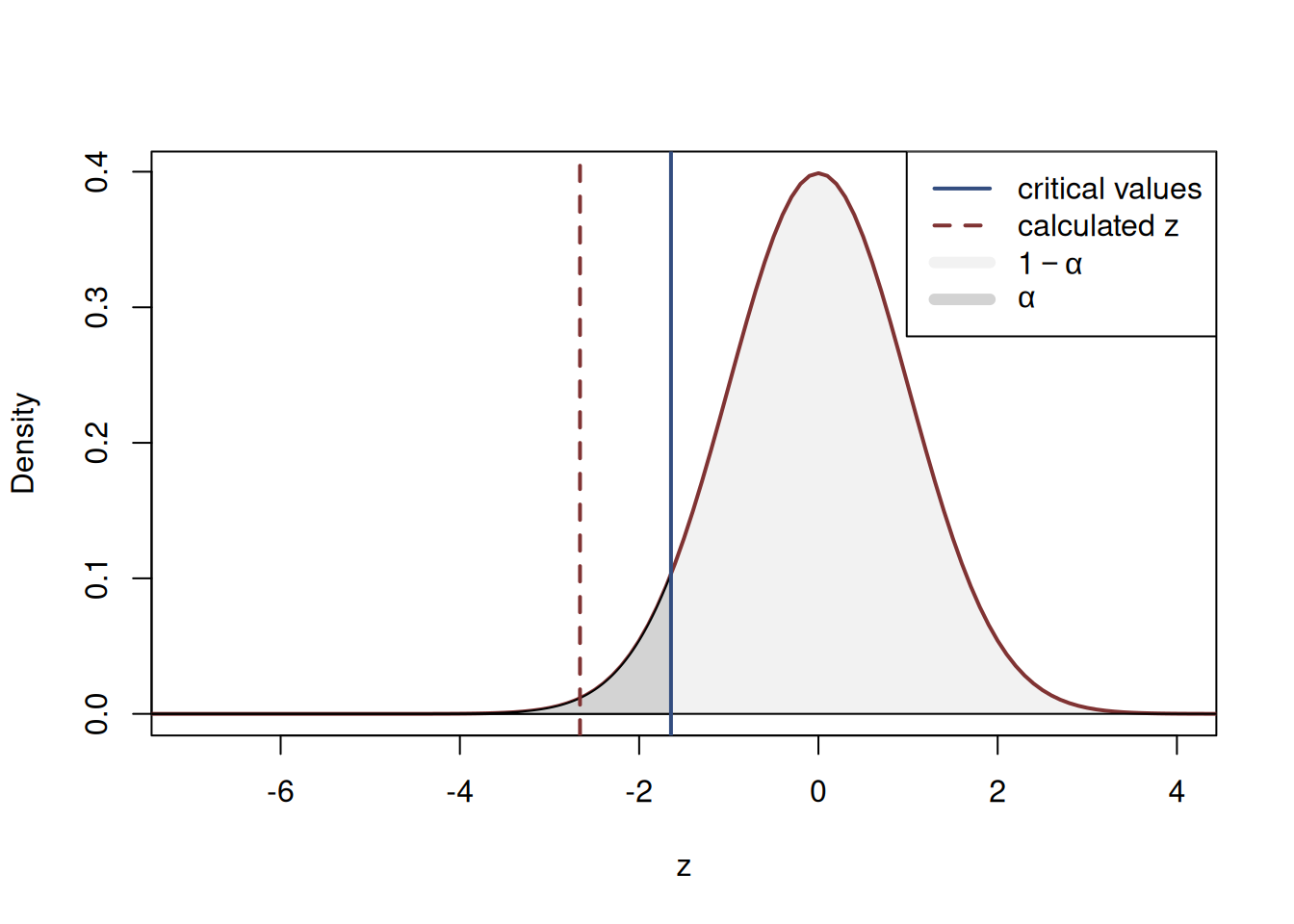
Figure 7.3: The process of hypothesis testing of one sided hypothesis (7.2).
The plot in Figure 7.3 shows the theoretical distribution of z-values, the 5% critical value and the calculated one. On the plot, we see that the calculated value lies in the tail of the distribution, which means that we can reject the null hypothesis on 5% significance level. The situation, when we correctly reject H\(_0\) in our example corresponds to the case, when the true distribution lies to the left of the assumed one as shown in Figure 7.4.
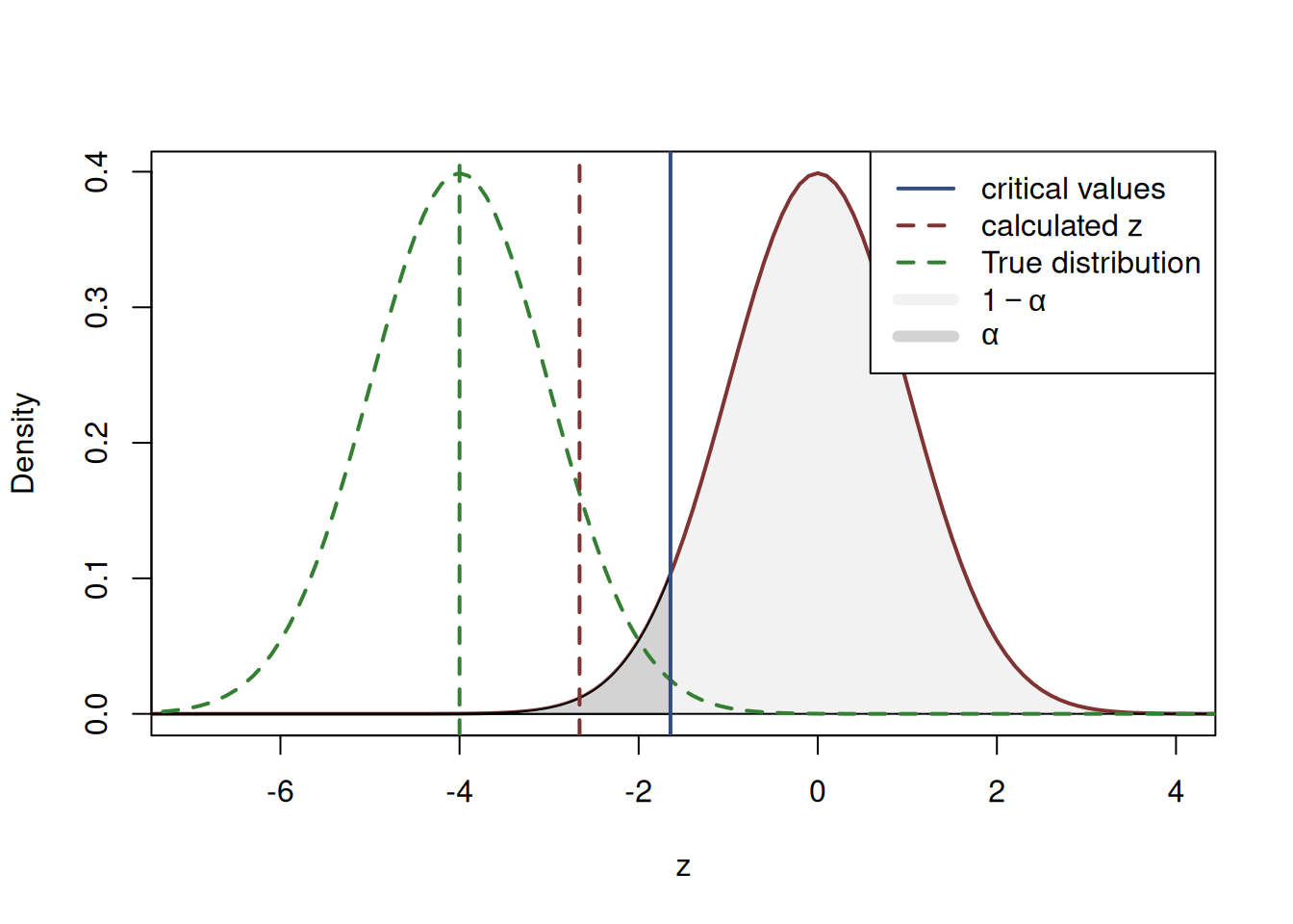
Figure 7.4: Hypothetical ‘true’ and the assumed distributions.
In the example of Figure 7.4 we consider a hypothetical situation, where the true mean is such that the standard normal distribution is centered around the value -4. In this example we correctly reject the wrong null hypothesis, which corresponds to the correct decision in Table 7.1 and the probability of this case is the “Power of a Test”. Visually, it corresponds to the surface of the “true” distribution to the left of the critical value that we have chosen in the beginning - any calculated value below this will lead to the rejection of H\(_0\) and thus to the correct decision. This is shown visually in Figure 7.5.
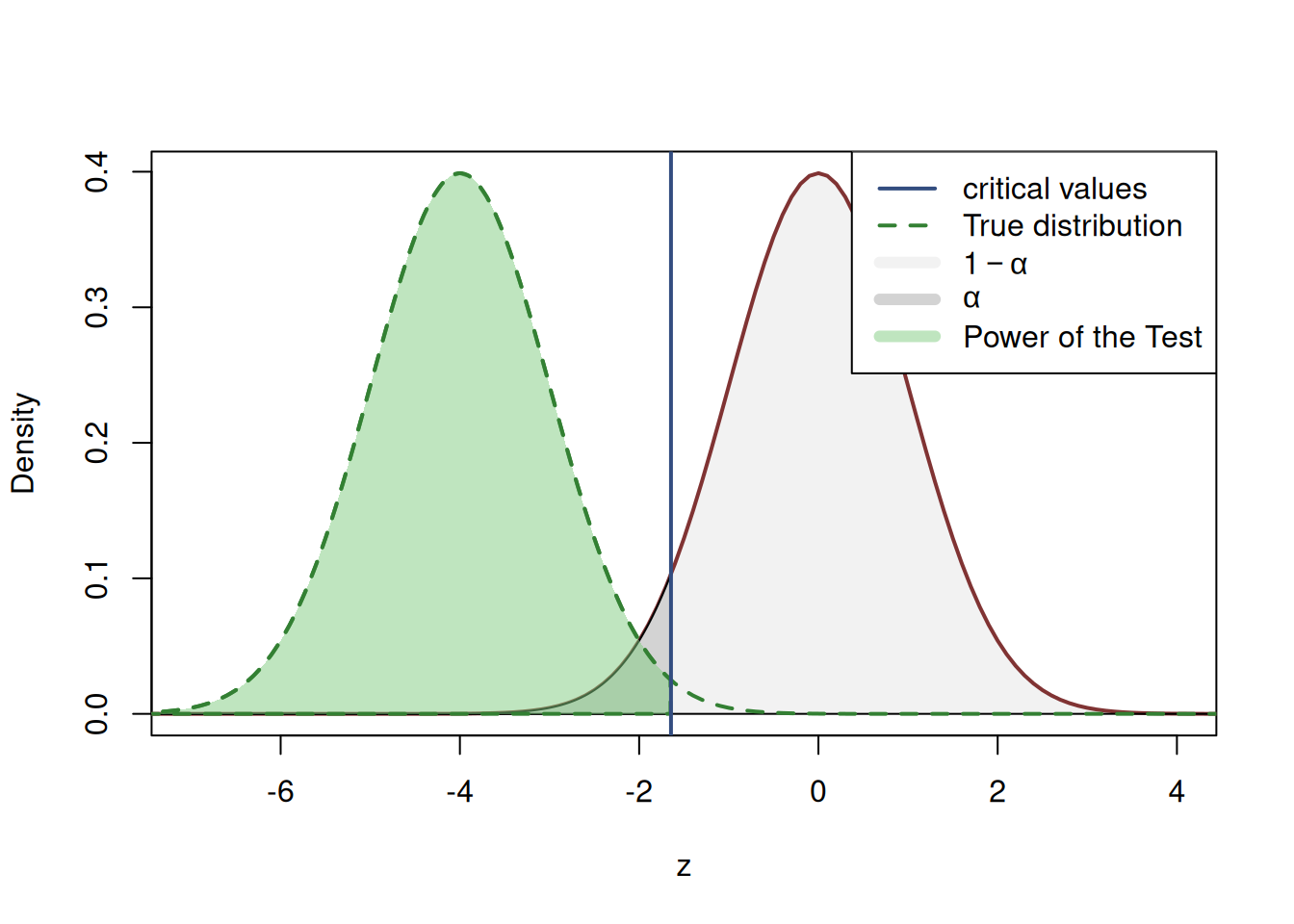
Figure 7.5: Power of the Test based on the hypothetical true value of \(\mu\).
The surface to the left of the critical value in Figure 7.5 is the Power of the Test for the example of a specific value of assumed \(\mu\). Given that we never know the true value, we could try other values, which would shift the distribution to the left or to the right, meaning either the increase or the decrease in power of the test. For example, the situation shown in Figure 7.6 corresponds to the smaller Power of the Test (because the surface of the distribution to the left is smaller than the surface of the distribution in Figure 7.5).
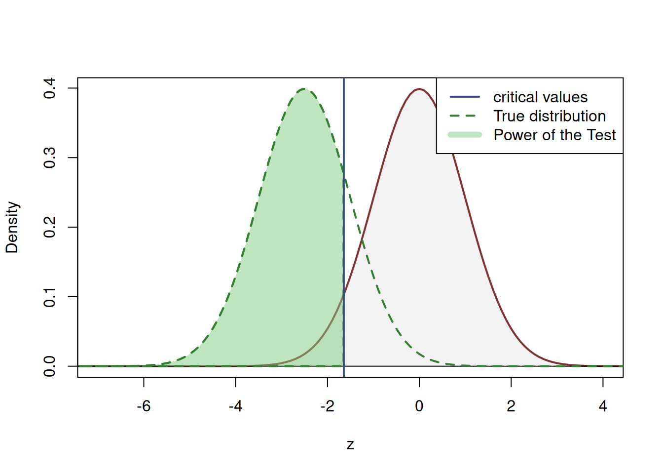
Figure 7.6: Power of the Test based on another hypothetical true value of \(\mu\).
Analysing Figures 7.5 and 7.6, we can already outline two factors impacting the power of a test:
- The location of the true mean. The further it is away to the tested one, the easier it is to detect the difference and reject the H\(_0\), which implies a higher power of a test;
- Significance level \(\alpha\). With the lower significance level, the critical value (vertical line in Figures 7.5 and 7.6) will be further to the left and thus the power of the test will be lower.
There are other factors, which are not as obvious as the two above. For example, if we did not know the true value of \(\sigma\), we would need to estimate it, and as a result we would need to use a less powerful t-test instead of the z-test. On smaller samples the critical value of the t-test is typically higher than the one from the z-test by absolute value. For example, in case of 36 observations, on 5% significance level it is equal to -1.6896, which is lower than the similar value of -1.6449 from the standard normal distribution. This means that if we used the t-test instead of the z-test in the example above, the vertical line on the plots in Figures 7.5 and 7.6 would be firther to the left of the one that we had. As a result, we would conclude that the power of the t-test is lower than the power of the z-test.
Furthermore, with the increase of the sample size the distribution of means tends to become narrower due to the Law of Large Numbers (see Section 6.2) and thus the power of tests grow, because the critical value moves closer to the centre of distribution.
7.3.2 Mathematical explantion
Moving from the visual explanation to the mathematical one, we can present the Power of a Test as the following probability: \[\begin{equation} \mathrm{P}(\text{reject H}_0 | \mathrm{H}_0 \text{ is wrong}) = 1 - \mathrm{P}(\text{Type II error}) = 1-\beta. \tag{7.3} \end{equation}\] As shown in the previous Subsection, the calculation of the Power of the Test is done based on the parameters of the specific test. In this Subsection, we continue with the same example as before and the same hypothesis: \[\begin{equation*} \mathrm{H}_0: \mu \geq 3, \mathrm{H}_1: \mu < 3. \end{equation*}\] For the example, we assume that the population standard deviation is known and is equal to \(\sigma=0.18\), that we work with a sample of 36 observations and that we use a 5% significance level to test the hypothesis. In this case, the test statistics is: \[\begin{equation} z = \frac{\bar{y}-3}{\sigma/\sqrt{n}} = \frac{\bar{y}-3}{0.03} , \tag{7.4} \end{equation}\] where \(\bar{y}\) is the sample mean. The rule for rejecting the null hypothesis in this situation is that if the calculated value \(z\) is lower than or equal to the critical one, which in our case (for the chosen 5% significance level) is -1.645: \[\begin{equation*} z = \frac{\bar{y}-3}{\sigma/\sqrt{n}} = \frac{\bar{y}-3}{0.03} \leq -1.645 \end{equation*}\] Solving this inequality for \(\bar{y}\), we will reject H\(_0\) if the sample mean is \[\begin{equation} \bar{y} \leq 3 -1.645 \times 0.03 = 2.95 . \tag{7.5} \end{equation}\] This can be interpreted as “we will fail to reject the null hypothesis in the cases, when the sample mean is greater than 2.95”. Now that we have this value, we can calculate the theoretical power of the test for a variety of cases. For example, we can see how powerful the test is in rejecting the wrong null hypothesis if the true mean is in fact equal to 2.87: \[\begin{equation} \begin{aligned} 1-\beta = & \mathrm{P}(\bar{y}\leq 2.95 | \mu=2.87) = \\ & \mathrm{P}\left(z \leq \frac{2.95 - 2.87}{0.03} \right) = \\ & \mathrm{P}\left(z \leq 2.67 \right) = \\ & 0.9962 \end{aligned} \tag{7.6} \end{equation}\] We could do similar calculations for other cases of the true mean and see how powerful the test is in those situations. In fact, we could create a power curve, showing how the power of the test changes in a variety of cases of hypothetical true mean. In R, this can be construct in the following way:
# Set all the parameters
yMean <- 3
yMeanSD <- 0.18 / sqrt(36)
levelSignigicance <- 0.05
zValue <- 3 + qnorm(levelSignigicance) * yMeanSD
# Vector of hypothetical population means
muValues <- seq(2.8,3.1,length.out=100)
# Vector of values for power curve
powerValues <- vector("numeric",100)

# Calculate the power values
powerValues <- pnorm((zValue - muValues)/yMeanSD)

# Plot the power curve
plot(muValues, powerValues, type="l",
     xlab=latex2exp::TeX("$\\mu$"),
     ylab="Power of the test")
# Add lines for the case of 1-beta=0.05
lines(rep(3,2),c(0,0.05), lty=3)
lines(c(0,3),rep(0.05,2), lty=3)
# And provide a description
text(3, 0.05+0.05,
     latex2exp::TeX("$\\alpha =1- \\beta =0.05$"),
     pos=4)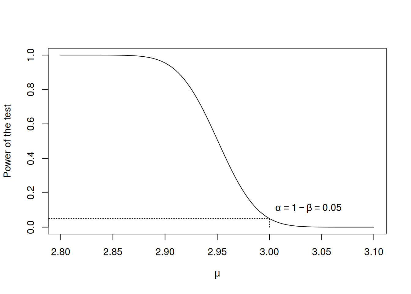
Figure 7.7: Power curve for the z-test in the example.
The plot in Figure 7.7 shows how powerful the z-test is for each specific value of population mean. We can see that the test becomes more powerful the further the true mean is away from the tested value (we chose 3 as the tested value). This means that it is easier for the test to detect the distance of the sample mean from the true value, when the true value is, for instance, 2.8 than in the case, when it is 2.95.
There is one specific point, where the power of the test coincides with the significance level. It is the case, when the population mean is indeed equal to 3. In this situation rejecting the null hypothesis would result in Type I error, which is equivalent to the significance level \(\alpha\), which we chose to be equal to 0.05.
In general, there are several things that influence the power of any statistical test:
- The value of the true parameter;
- The significance level;
- The sample size;
- The amount of information available for the test.
The element (1) is depicted on the plot in Figure 7.7. If we conduct the test about the wrong value of the true mean, then the distance from it will impact the power: the further it is away, the more powerful the test will be, being able to tell the difference between the sample mean and the true mean.
The element (2) will define the critical value of a statistical test, and in general the smaller the significance level is, the less powerful the test will be, as we will not be able to spot small discrepancies from the true mean.
The larger the sample size (element (3)), the more powerful the test becomes in general. In our example, we can see that from the equation (7.4), where the sample size \(n\) is in the denominator of the denominator. The higher values of \(n\) will lead to the higher values of \(z\) and as a result, the higher chance of rejecting the H\(_0\) if it is wrong. Figure 7.8 demonstrates how the power curve changes with the increase of the sample size. we see that the power of the test increases much faster with the decrease of the hypothetical value of \(\mu\), when the sample size is large (for example, \(n=1000\)) than in the case of small samples (e.g., \(n=25\)).
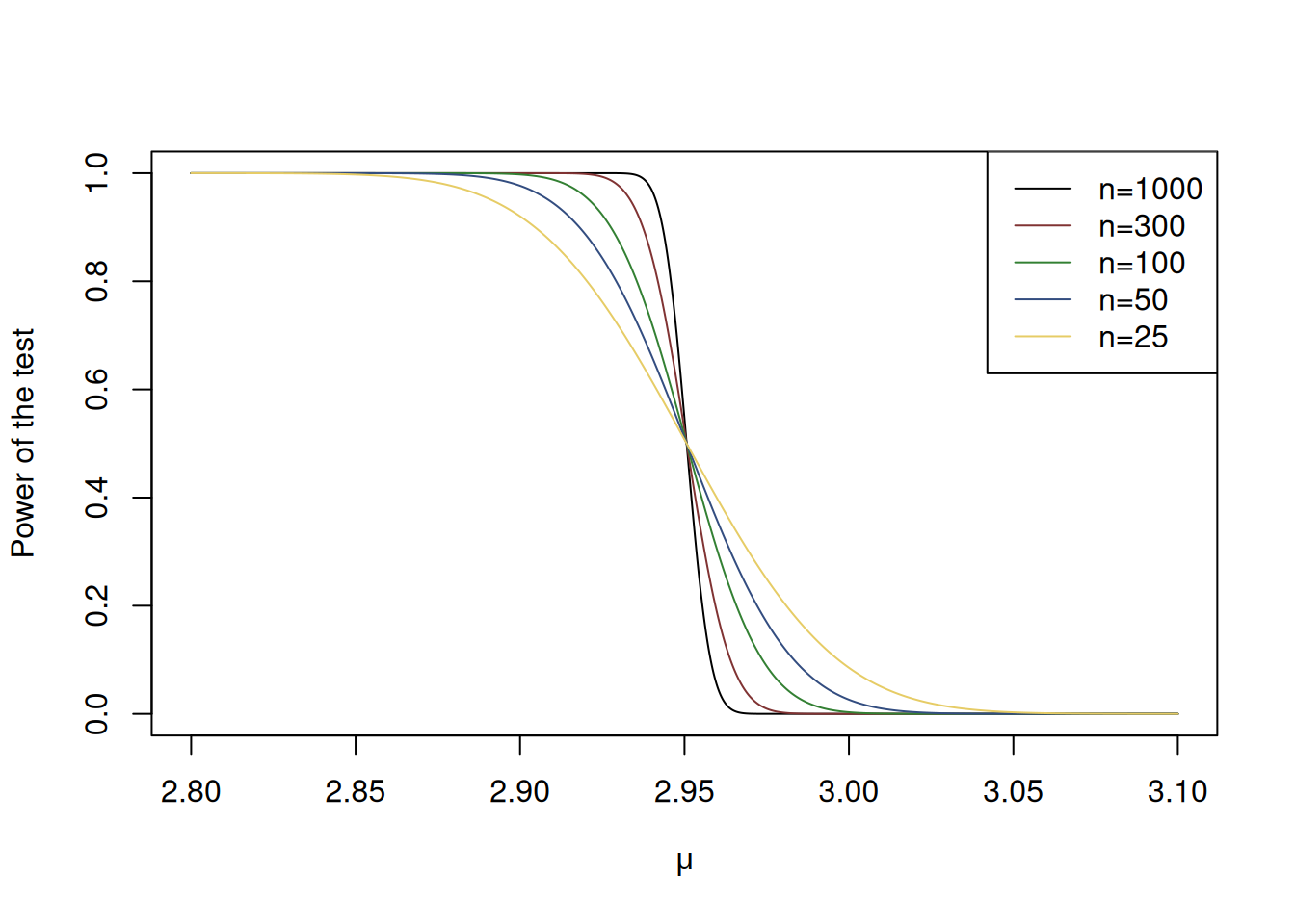
Figure 7.8: Power curves with different sample sizes.
Finally, the more general point about the “amount of information” applies to the selection between the tests. In the Section 8 we will discuss a variety of tests and we will discuss the conditions under which some of them are more powerful than the others. But in general the rule is: the more a priori information you can provide to the test, the easier it becomes to detect deviations from the tested value, because the uncertainty caused by estimation of additional parameters is decreased in this case.
7.3.3 Expected power of a test
As discussed in the previous subsections, the power of a test is calculated for each specific value of \(\mu\), measuring the probability of rejecting the wrong hypothesis for the specific parameters. This approach has a limitation, because typically we do not know the true value of \(\mu\), and sometimes selecting the correct one is challenging. One of the solutions in this case is calculating the expected power of a test or Assurance (O’Hagan et al., 2005), which is the expectation of the probability (7.3) for all possible values of \(\mu\) for which the hypothesis would be correctly rejected. In a special case, when \(\mu\) can only take discrete values, this can be roughly represented as a mean of powers for all values of \(\mu\) that are lower than the value \(\mu^*\) that corresponds to the critical one (in our example in Subsection 7.3.2 \(\mu^*\) was equal to \(2.95\)): \[\begin{equation} \mathrm{E}(\mathrm{P}(\text{reject wrong }\mathrm{H}_0)) = \sum_{\mu_j<\mu^*} \mathrm{P}(\text{reject }\mathrm{H}_0 | \mu=\mu_j) \times \mathrm{P}(\mu=\mu_j) . \tag{7.7} \end{equation}\] Note that we sum up all the values up until \(\mu^*\), because the value higher than that would imply that we fail to reject the correct hypothesis. Note that in reality \(\mu\) or any other parameter of distribution is typically continuous, which means that a probability density function should be used instead of probabilities and an integral should be used instead of the sum in (7.7), i.e.: \[\begin{equation} \mathrm{E}(\mathrm{P}(\text{reject wrong }\mathrm{H}_0)) = \int_{-\infty}^{\mu^*} \mathrm{P}(\text{reject }\mathrm{H}_0 | \mu=x) \times f(x)dx . \tag{7.8} \end{equation}\]
Remark. Note that the integration is done until \(\mu^*\), covering the values, where the hypothesis would be correctly rejected. In the example discussed in Subsection 7.3.2, we calculated in equation (7.5) that \(\mu^*=2.95\). If we had a different null hypothesis, we would do integration differently. For example, in case of \(\mathrm{H}_0: \mu \leq 3\), the integration would be done from 2.95 to \(\infty\).
The calculation of the assurance in some cases can be done analytically. For example, O’Hagan et al. (2005) derive formulae for normal distribution for several tests. However, the analytical solution in some cases might be either too complicated, or unavailable. In these situations, the integration can be done numerically, for example, using Monte-Carlo simulations.
Finally, in practice, the assurance is used to determine the sample size for trials. The canonical example of application is deciding how many participants are needed to establish the effectiveness of a medical treatment, by setting the desired assurance to the pre-specified value.