12.2 Confidence intervals of parameters
Given that the estimates of parameters have some uncertainty associated with them, as discussed in the introduction to this chapter, it makes sense to capture that uncertainty so that decision makers can have a better understanding about the observed effects. Covariance matrix discussed in Section 12.1 captures that uncertainty, but it is hard to make any decision based on it.
A simpler way to do that is to construct confidence intervals in a similar way to how we did that in Section 6.5. Visually, this process is shown in Figure 12.3, which continues the example we discussed earlier.
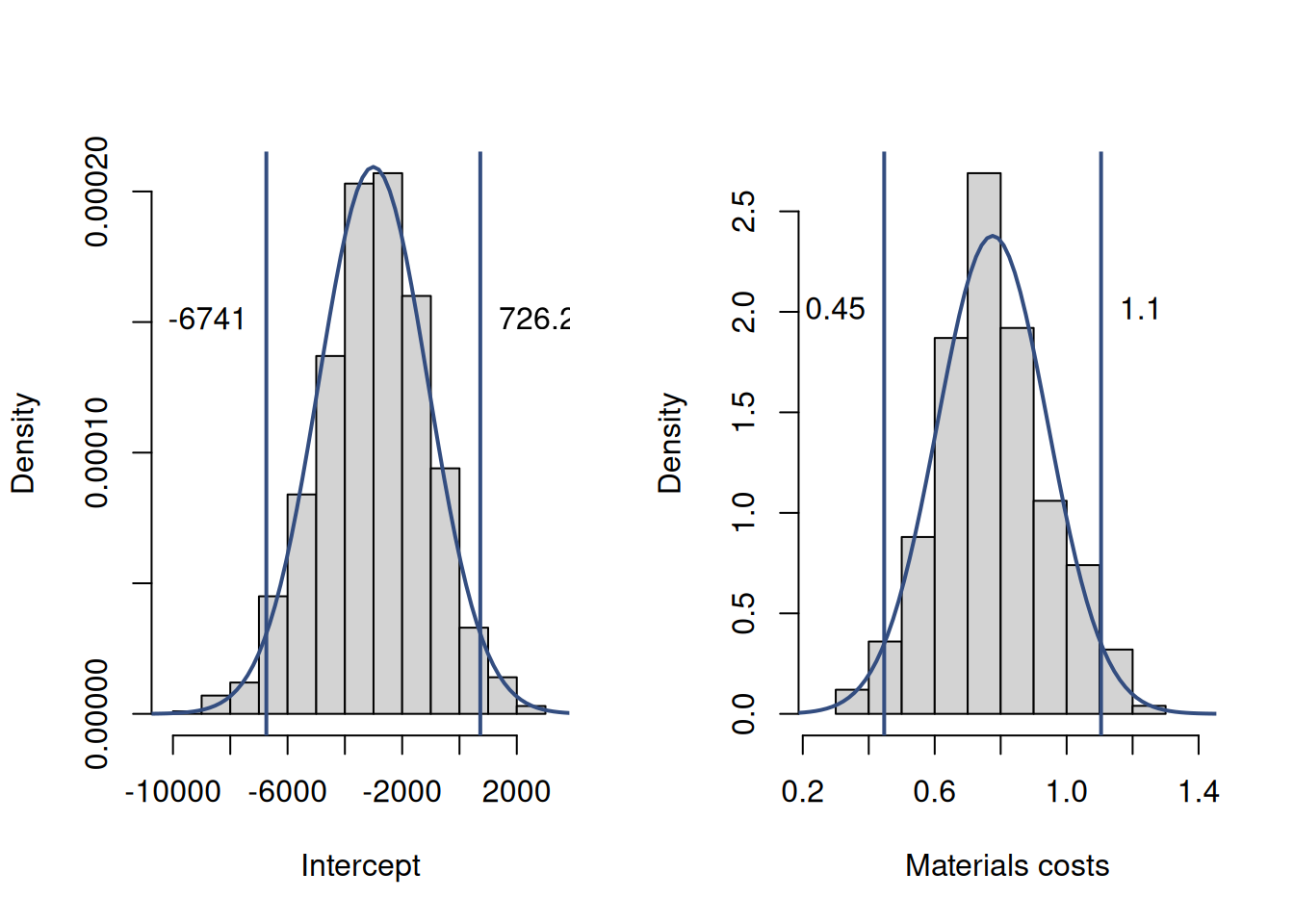
Figure 12.3: Parameter uncertainty in the estimated model
Figure 12.3 demonstrates the bootstrapped distributions of parameters (as before), together with the Normal probability density functions on top of them and vertical lines at the tails that represent the confidence bounds. The idea behind this is that due to the Central Limit Theorem (Section 6.3) we can assume that estimates of parameters follow the Normal distribution with some mean and variance, and based on that we can get the quantiles, thus inferring, for example, that the true intercept will lie between -5199.78 and 6444.31 in the 95% of the cases, if we repeat the resampling experiment many times.
The interpretation of the confidence interval is exactly the same as in the simpler case discussed in the Section 6.5. The formula for it is slightly different, because it is constructed for the parameters of the model rather than the mean of the sample, but the logic is exactly the same: \[\begin{equation} \beta_i \in (b_i + t_{\alpha/2}(n-k) s_{b_i}, b_i + t_{1-\alpha/2}(n-k) s_{b_i}), \tag{12.13} \end{equation}\] where \(s_{b_i}\) is the standard error of the parameter \(b_i\). An important note to make is that, as usual with confidence interval construction, we can use the Normal distribution only in the case when the variance of parameters is known. In reality, it is not, so, as discussed in Section 6.5, we need to use the Student’s t distribution. This is why we have \(t_{\alpha/2}(n-k)\) in the equation (12.13) above.
Remark. The important note is that in order to be able to use the formula (12.13), we need the Central Limit Theorem to hold. If it does not, then the estimates of parameters would not follow the Normal distribution, and the Student’s t-statistics would not be appropriate to calculate the interval.
To calculate the confidence interval, using the equation (12.13), we need to know several things:
- Significance level \(\alpha\) - we define it either based on our preferences or on the task at hand. This should be selected prior to construction of the interval. The typical one is 5%, mainly because the standard human has five fingers on a hand;
- The value of the estimated parameter \(b_i\). We get it after using the Least Squares, any statistical software can give us the estimate.
- Standard error (or deviation) of the parameter. This is obtained from the covariance matrix of parameters discussed in Section 12.1.
- Number of degrees of freedom \(n-k\), which can be easily calculated based on the sample size \(n\) and the number of estimated parameters \(k\).
- Student’s t statistics. We get it from statistical tables or the software, given the significance level \(\alpha\) and the number of degrees of freedom \(n-k\) above.
Example 12.1 Consider construction of the interval for the slope parameter for the variable materials from the regression we discussed earlier. In our case, we know the following:
- \(\alpha=0.05\) because we decided to produce the 95% confidence interval. We could choose the other value, which would result in the interval of a different width;
- The value of the parameter \(b_1\) is 0.8706;
- To get the variance of the parameter, we can use the formula discussed in Section 12.1. In R, we can get the variance of the parameter for the
materials(second parameter in the model) via thevcov()function, like this:
## [1] 0.09681792Based on that, we can say that the standard error of the parameter (square root of the variance) is approximately 0.3112.
4. We estimated five parameters (four for variables and an intercept), so \(k=5\), and the sample size \(n\) was 61, which means that in our model has \(n-k=61-5=56\) degrees of freedom.
5. To get the Student’s t statistics correctly, we need to split the significance level \(\alpha\) into two equal part, meaning that we expect to have 2.5% of values below the lower bound and another 2.5% of values above the upper one. So, we will calculate it for \(\alpha/2=0.025\) and \(1-\alpha/2=0.975\) with \(n-k=56\). In R, we can use the qt() function in the following way:
## [1] -2.003241 2.003241Taking all these values and inserting them in the formula (12.13), we should get the two numbers, representing the lower and the upper bounds of the 95% confidence interval respectively: (0.2472,1.494)
In R, the confidence interval can be obtained directly via the confint() function, and it should be close to what we obtained above, but not exactly the same due to rounding:
##                  S.E.       2.5%     97.5%
## (Intercept) 4337.3590 -8074.4514 9303.0968
## materials      0.3112     0.2473    1.4939
## size           0.6989    -0.0529    2.7471
## projects       3.7971    -9.1986    6.0144
## year           2.1621    -4.4915    4.1711
The confidence interval for materials above shows, for example, that if we repeat the construction of interval many times on different samples of data, the true value of parameter will lie in 95% of cases between 0.2473 and 1.4939. This gives us an idea about the real effect in the population and how certain we are about it.
We can also present all of this in the following summary (this is based on the alm() model, the other functions will produce different outputs):
## Response variable: overall
## Distribution used in the estimation: Normal
## Loss function used in estimation: MSE
## Coefficients:
##             Estimate Std. Error Lower 2.5% Upper 97.5%
## (Intercept) 614.3227  4337.3590 -8074.4514   9303.0968
## materials     0.8706     0.3112     0.2473      1.4939 *
## size          1.3471     0.6989    -0.0529      2.7471
## projects     -1.5921     3.7971    -9.1986      6.0144
## year         -0.1602     2.1621    -4.4915      4.1711
##
## Error standard deviation: 43.4158
## Sample size: 61
## Number of estimated parameters: 5
## Number of degrees of freedom: 56
## Information criteria:
##      AIC     AICc      BIC     BICc
## 639.9341 641.4896 652.5993 655.7967
This summary provides all the necessary information about the model and the estimates of parameters:
- their mean values are in the column “Estimate”,
- their standard errors (square roots of the variances) are in “Std. Error”,
- the bounds of confidence interval are in the last two columns,
- and, finally, a star drawn next to the interval if it does not contain zero.
If we have that star, then this indicates that we are certain on the selected confidence level (95% in our example) about the sign of the parameter and that the effect indeed exists. We can regulate the confidence level by defining the level parameter. For example, if we want the 99% one, we should add level=0.99 in the summary: