15.1 Model is correctly specified

This book is in Open Review. I want your feedback to make the book better for you and other readers. To add your annotation, select some text and then click the on the pop-up menu. To see the annotations of others, click the button in the upper right hand corner of the page

This is one of the fundamental group of assumptions, which can be summarised as “we have included everything necessary in the model in the correct form”. It implies that:

15.1.1 Omitted variables

If there are some important variables that we did not include in the model, then the estimates of the parameters might be biased and in some cases quite seriously (e.g. positive sign instead of the negative one). A classical example of model with omitted important variables is simple linear regression, which by definition includes only one explanatory variable. Making decisions based on such model might not be wise, as it might mislead about the significance and sign of effects. Yes, we use simple linear regression for educational purposes, to understand how the model works and what it implies, but it is not sufficient on its own. Finally, when it comes to forecasting, omitting important variables is equivalent to underfitting the data, ignoring significant aspects of the model. This means that the point forecasts from the model might be biased (systematic under or over forecasting), the variance of the error term will be higher than needed, which will result in wider than necessary prediction interval.

In some cases, it is possible to diagnose the violation of this assumption. In order to do that an analyst needs to analyse a variety of plots of residuals vs fitted, vs time (if we deal with time series), and vs omitted variables. Consider an example with mtcars data and a simple linear regression:

mtcarsSLR <- alm(mpg~wt, mtcars, loss="MSE")

Based on the preliminary analysis that we have conducted in Sections 5 and 9, this model omits important variables. And there are several basic plots that might allow us diagnosing the violation of this assumption.

par(mfcol=c(1,2))
plot(mtcarsSLR,c(1,2))

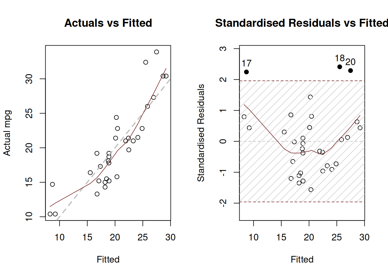
Figure 15.1: Diagnostics of omitted variables.

Figure 15.1 demonstrates actuals vs fitted and fitted vs standardised residuals. The standardised residuals are the residuals from the model that are divided by their standard deviation, thus removing the scale. What we want to see on the first plot in Figure 15.1, is for all the point lie around the grey line and for the LOWESS line to coincide with the grey line. That would mean that the relations are captured correctly and all the observations are explained by the model. As for the second plot, we want to see the same, but it just presents that information in a different format, which is sometimes easier to analyse. In both plot of Figure 15.1, we can see that there are still some patterns left: the LOWESS line has a u-shaped form, which in general means that something is wrong with model specification. In order to investigate if there are any omitted variables, we construct a spread plot of residuals vs all the variables not included in the model (Figure 15.2).

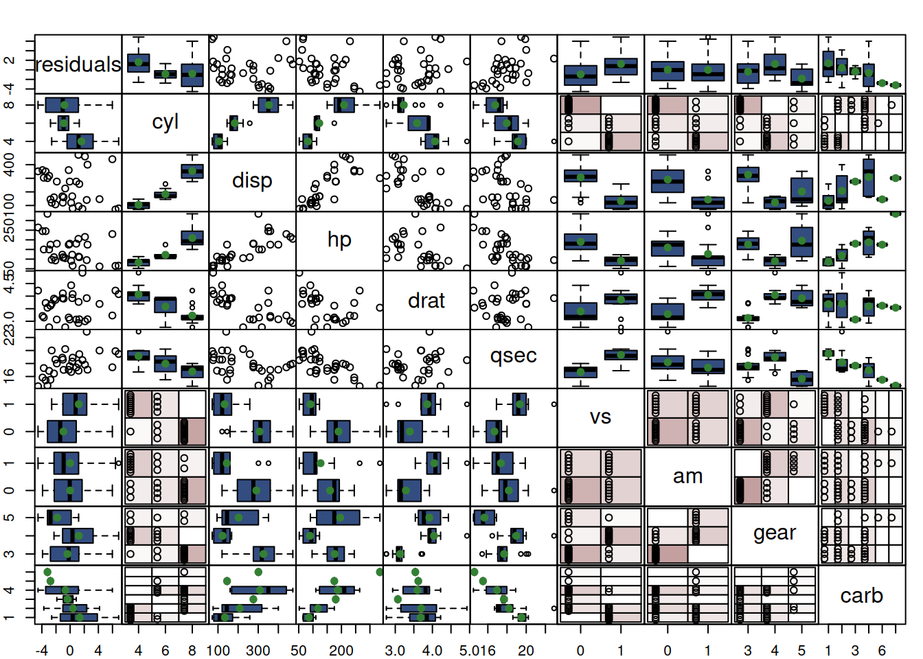
spread(data.frame(residuals=resid(mtcarsSLR), mtcars[,-c(1,6)]))

Figure 15.2: Diagnostics of omitted variables.

What we want to see in Figure 15.2 is the absence of any patterns in plots of residuals vs variables. However, we can see that there are still many relations. For example, with the increase of the number of cylinders, the mean of residuals decreases. This might indicate that the variable is needed in the model. And indeed, we can imagine a situation, where mileage of a car (the response variable in our model) would depend on the number of cylinders because the bigger engines will have more cylinders and consume more fuel, so it makes sense to include this variable in the model as well.

Note that we do not suggest to start modelling from simple linear relation! You should construct a model that you think is suitable for the problem, and the example above is provided only for illustrative purposes.

15.1.2 Redundant variables

If there are redundant variables that are not needed in the model, then the estimates of parameters and point forecasts might be unbiased, but inefficient. This implies that the variance of parameters can be lower than needed and thus the prediction intervals will be narrower than needed. There are no good instruments for diagnosing this issue, so judgment is needed, when deciding what to include in the model.

15.1.3 Transformations

This assumption implies that we have taken all possible non-linearities into account. If, for example, instead of using a multiplicative model, we apply an additive one, the estimates of parameters and the point forecasts might be biased. This is because the model will produce linear trajectory of the forecast, when a non-linear one is needed. This was discussed in detail in Section 14. The diagnostics of this assumption is similar to the diagnostics shown above for the omitted variables: construct actuals vs fitted and residuals vs fitted in order to see if there are any patterns in the plots. Take the multiple regression model for mtcars, which includes several variables, but is additive in its form:

mtcarsALM01 <- alm(mpg~wt+qsec+am, mtcars, loss="MSE")

Arguably, the model includes important variables (although there might be some others that could improve it), but the residuals will show some patterns, because the model should be multiplicative (see Figure 15.3), because mileage should not reduce linearly with increase of those variables. In order to understand that, ask yourself, whether the mileage can be negative and whether weight and other variables can be non-positive (a car with \(wt=0\) just does not exist).

par(mfcol=c(1,2))
plot(mtcarsALM01,c(1,2))

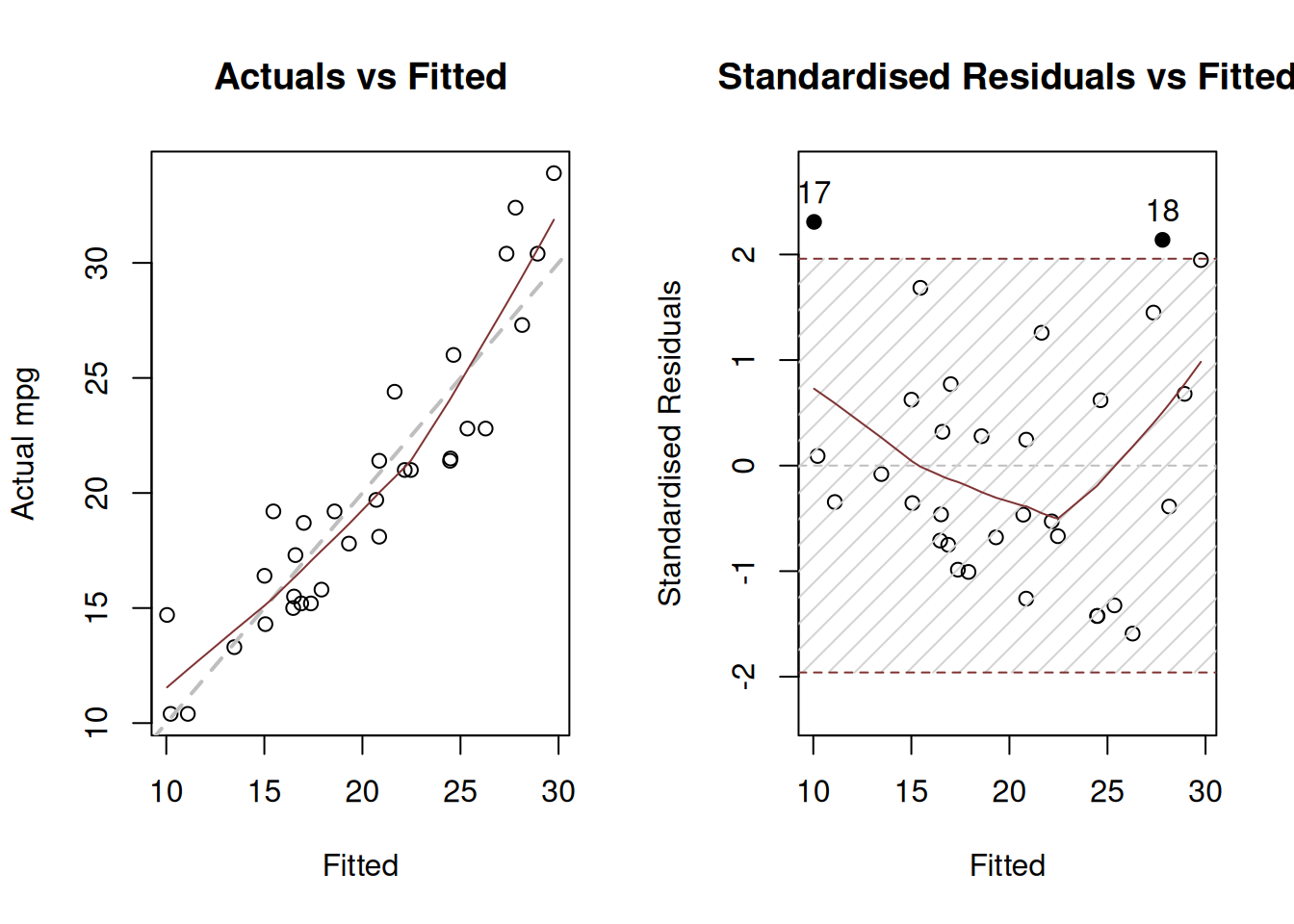
Figure 15.3: Diagnostics of necessary transformations in linear model.

Figure 15.3 demonstrates the u-shaped pattern in the residuals, which is one of the indicators of a wrong model specification, calling for a non-linear transformation. We can try a model in logarithms:

mtcarsALM02 <- alm(log(mpg)~log(wt)+log(qsec)+am, mtcars, loss="MSE")

And see what would happen with the diagnostics of the model in logarithms:

par(mfcol=c(1,2))
plot(mtcarsALM02,c(1,2))

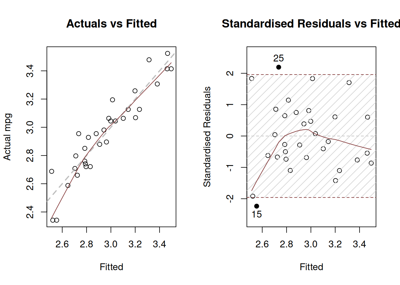
Figure 15.4: Diagnostics of necessary transformations in log-log model.

Figure 15.4 demonstrates that while the LOWESS lines do not coincide with the grey lines, the residuals do not have obvious patterns. The fact that the LOWESS line starts from below, when fitted values are low in our case only shows that we do not have enough observations with low actual values. As a result, LOWESS is impacted by 2 observations that lie below the grey line. This demonstrates that LOWESS lines should be taken with a pinch of salt and we should abstain from finding patterns in randomness, when possible. Overall, the log-log model is more appropriate to this data than the linear one.

15.1.4 Outliers

In a way, this assumption is similar to the first one with omitted variables. The presence of outliers might mean that we have missed some important information, implying that the estimates of parameters and forecasts would be biased. There can be other reasons for outliers as well. For example, we might be using a wrong distributional assumption. If so, this would imply that the prediction interval from the model is narrower than necessary. The diagnostics of outliers comes to producing standardised residuals vs fitted, to studentised vs fitted and to Cook’s distance plot. While we are already familiar with the first one, the other two need to be explained in more detail.

Studentised residuals are the residuals that are calculated in the same way as the standardised ones, but removing the value of each residual. For example, the studentised residual on observation 25 would be calculated as the raw residual divided by standard deviation of residuals, calculated without this 25th observation. This way we diminish the impact of potential serious outliers on the standard deviation, making it easier to spot the outliers.

As for the Cook’s distance, its idea is to calculate measures for each observation showing how influential they are in terms of impact on the estimates of parameters of the model. If there is an influential outlier, then it would distort the values of parameters, causing bias.

par(mfcol=c(1,2))
plot(mtcarsALM02,c(2,3))

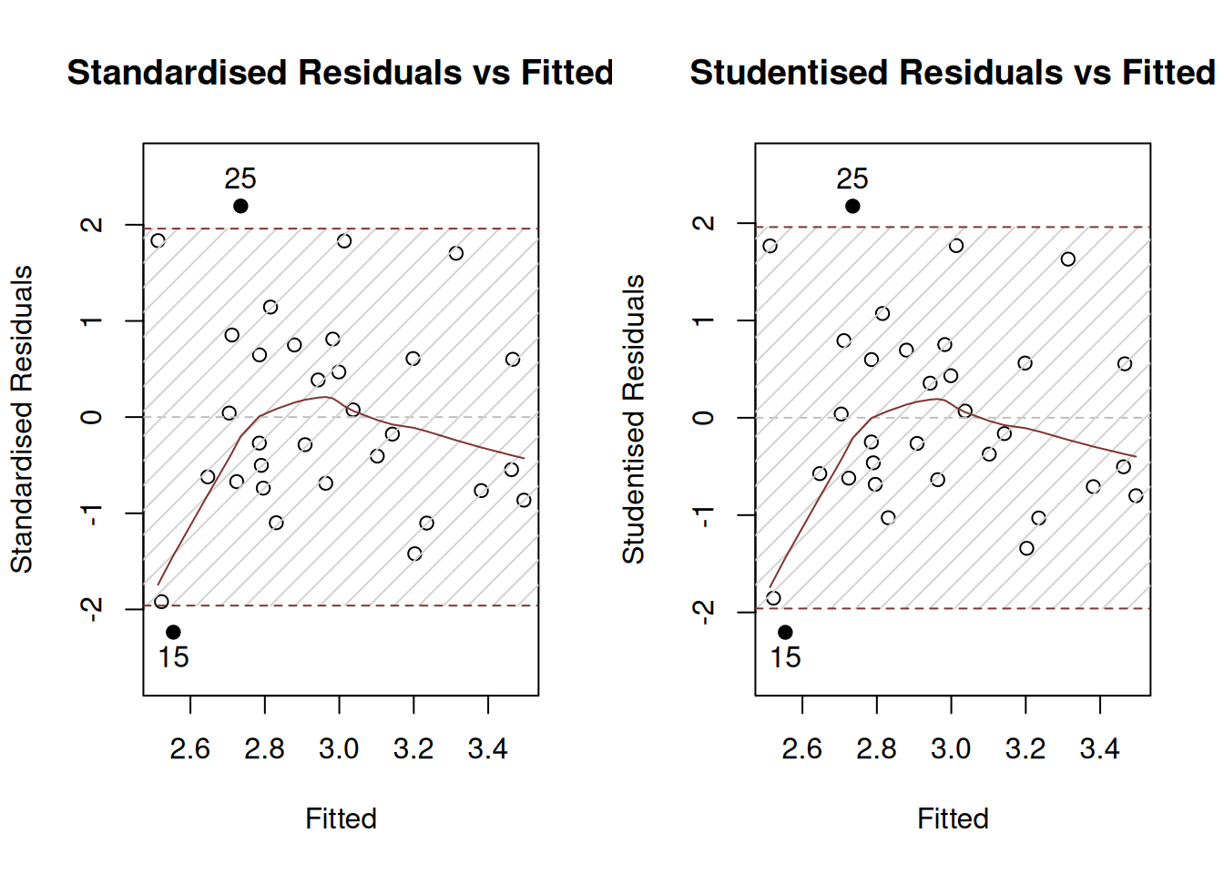
Figure 15.5: Diagnostics of outliers.

Figure 15.5 demonstrates standardised and studentised residuals vs fitted values for the log-log model on mtcars data. We can see that the plots are very similar, which already indicates that there are no strong outliers in the residuals. The bounds produced on the plots correspond to the 95% prediction interval, so by definition it should contain \(0.95\times 32 \approx 30\) observations. Indeed, there are only two observations: 15 and 25 - that lie outside the bounds. Technically, we would suspect that they are outliers, but they do not lie far away from the bounds and their number meets our expectations, so we can conclude that there are no outliers in the data.

plot(mtcarsALM02,12)

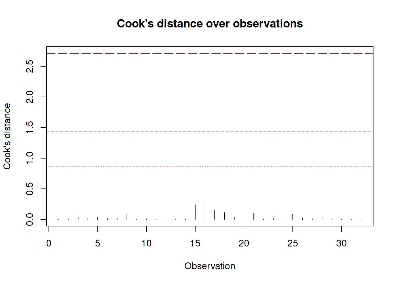
Figure 15.6: Cook’s distance plot.

Finally, we produce Cook’s distance over observations in Figure 15.6. The x-axis says “Time”, because alm() function is tailored for time series data, but this can be renamed into “observations”. The plot shows how influential the outliers are. If there were some significantly influential outliers in the data, then the plot would draw red lines, corresponding to 0.5, 0.75 and 0.95 quantiles of Fisher’s distribution, and the line of those outliers would be above the red lines. Consider the following example for demonstration purposes:

mtcarsData[28,6] <- 4
mtcarsALM03 <- alm(log(mpg)~log(wt)+log(qsec)+am, mtcarsData, loss="MSE")

This way, we intentionally create an influential outlier (the car should have the minimum weight in the dataset, and now it has a very high one).

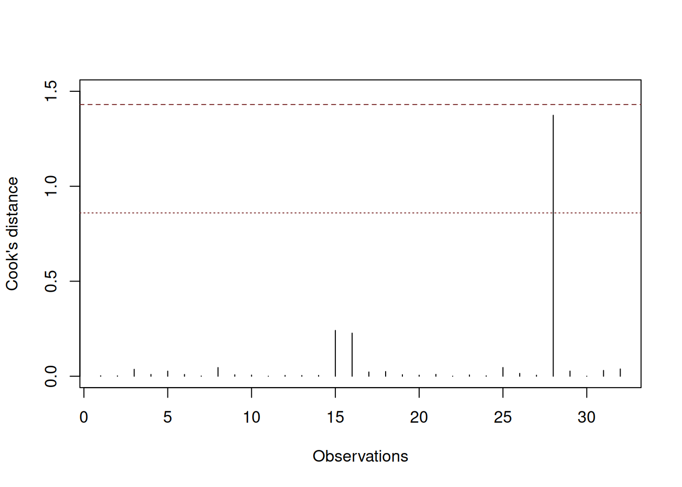
plot(mtcarsALM03, 12, ylim=c(0,1.5), xlab="Observations", main="")

Figure 15.7: Cook’s distance plot for the data with influential outlier.

Figure 15.7 shows how Cook’s distance will look in this case - it detects that there is an influential outlier, which is above the norm. We can compare the parameters of the new and the old models to see how the introduction of one outlier leads to bias in the estimates of parameters:

rbind(coef(mtcarsALM02),
      coef(mtcarsALM03))

##      (Intercept)    log(wt) log(qsec)         am
## [1,]   1.2095788 -0.7325269 0.8857779 0.05205307
## [2,]   0.1382442 -0.4852647 1.1439862 0.21406331