8.2 One-sample test about variance
Another example of a situation that could be potentially interesting in practice is when we are not sure about the estimated variance of a distribution. We might want to understand, whether the variance in population is similar to the value we obtained based on our sample. For illustrative purposes, consider the continued example with the height of humans. After collecting the sample of 30 observations, it was found that the variance of height is 100. However, based on previous survey, we know that the population variance of the height is 121. We want to know whether the in-sample estimate of variance is significantly lower from the population one on 1% significance level. This hypothesis can be formulated as: \[\begin{equation*} \mathrm{H}_0: \sigma^2 \geq 121, \mathrm{H}_1: \sigma^2 < 121 . \end{equation*}\] where \(\sigma^2\) is the population variance. The conventional test for this hypothesis is the Chi-squared test (\(\chi^2\)). This is a parametric test, which means that it relies on distributional assumptions. However, unlike the test about the mean from the Section 8.1 (which assumed that CLT holds, see Section 6.3), the Chi-squared test relies on the assumption about the random variable itself: \[\begin{equation*} y_j \sim \mathcal{N}(\mu, \sigma^2) , \end{equation*}\] which means that (as discussed in Section 8.1.1): \[\begin{equation*} z_j = \frac{y_j - \mu}{\sigma} \sim \mathcal{N}(0, 1) . \end{equation*}\] Coming back to the variance, we would typically use the following formula to estimate it in sample: \[\begin{equation*} \mathrm{V}\left( y \right) = \frac{1}{n-1} \sum_{j=1}^n \left(y_j - \bar{y} \right)^2, \end{equation*}\] where \(\bar{y}\) is an unbiased, efficient and consistent estimate of \(\mu\) (Section 6.4). If we divide the variance by the true value of the population one, we will get the following: \[\begin{equation*} \frac{\mathrm{V}\left( y \right)}{\sigma^2} = \frac{1}{n-1} \sum_{j=1}^n \frac{\left(y_j - \bar{y} \right)^2}{\sigma^2}, \end{equation*}\] or after multiplying it by \(n-1\): \[\begin{equation} \chi^2 = (n-1) \frac{\mathrm{V}\left( y \right)}{\sigma^2} = \sum_{j=1}^n z_j^2 . \tag{8.3} \end{equation}\] Given the assumption of normality of the random variable \(z_j\), the variable (8.3) will follow the Chi-squared distribution with \(n-1\) degrees of freedom (this is the definition of the Chi-squared distribution). This property can be used to test a statistical hypothesis about the variance.
The hypothesis testing itself is done using the same procedure as before (Section 7.1). After formulating the hypothesis and selecting the significance level, we use the formula (8.3) to get the calculated value: \[\begin{equation*} \chi^2 = (30-1) \times \frac{100}{121} \approx 23.97 \end{equation*}\] Given that the alternative hypothesis in our example is “lower than”, we should compare the obtained value with the critical one from the left tail of the distribution, which on 1% significance level is:
## [1] 14.25645Comparing the critical and calculated values (\(23.97>14.26\)), we conclude that we fail to reject the null hypothesis. This means that the sample variance is not statistically different from the population one. The test of this hypothesis is shown visually in Figure 8.2, which shows that the calculated value is not in the tail of the distribution (thus “fail to reject”).
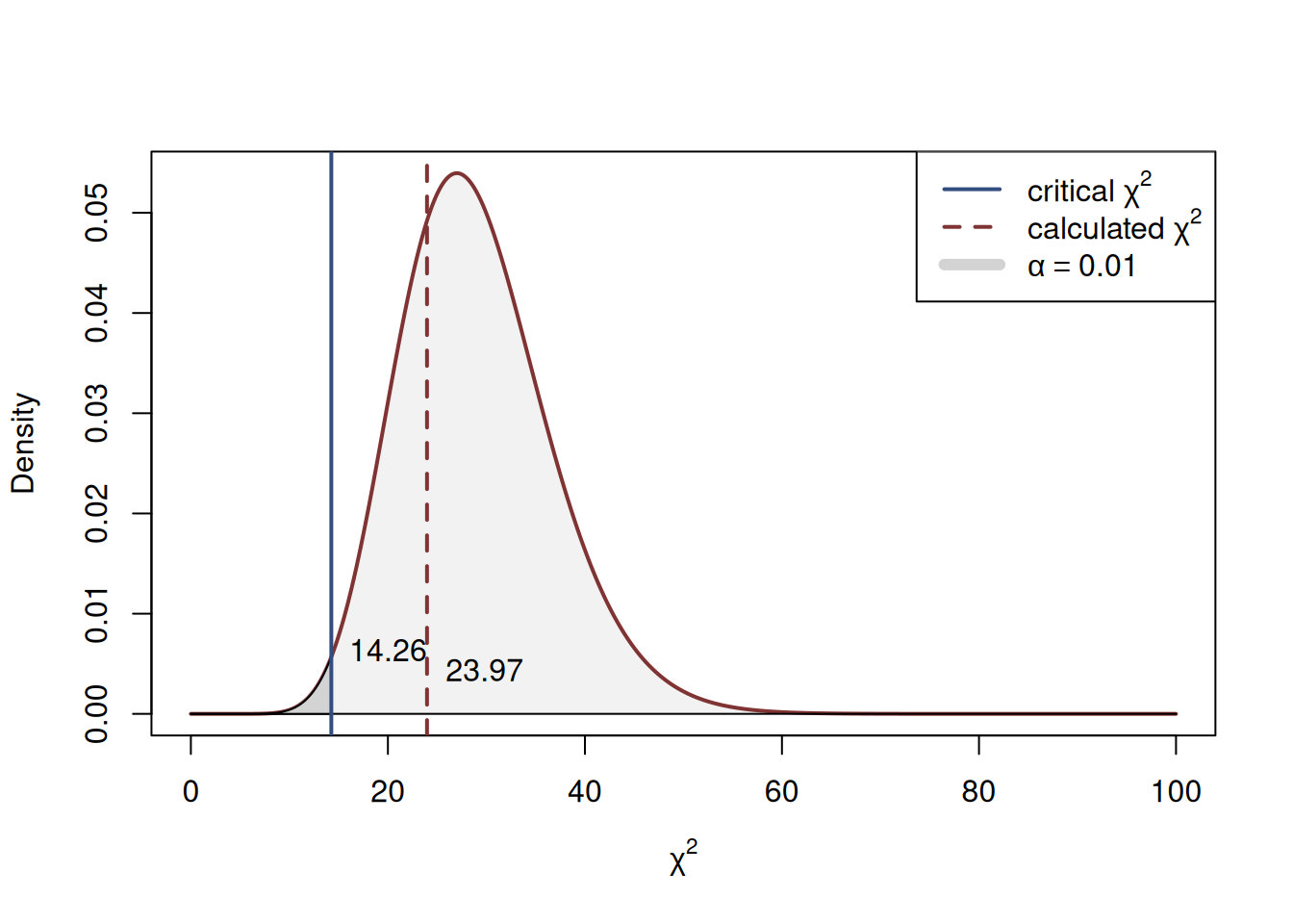
Figure 8.2: The process of hypothesis testing in Chi-squared distribution (one-tailed case).
A thing to keep in mind about the Chi-square distribution is that it is in general asymmetric (it converges to normal with the increase of the sample size, see discussion in Chapter 4). This means that if the alternative hypothesis is formulated as “not equal”, the absolutes of critical values for the left and right tails will differ. This situation is shown in Figure 8.3 with the example of 5% significance level, which is split into two equal parts of 2.5% with critical values of 16.05 and 45.72.
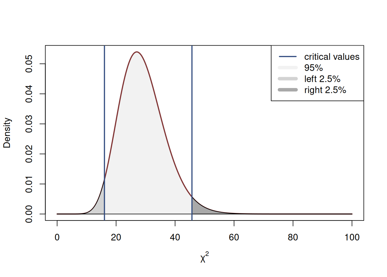
Figure 8.3: The process of hypothesis testing in Chi-squared distribution (two-tailed case).
The surfaces in the tails in Figure 8.3 are equal, but because of the asymmetry of distribution they look different.
Remark. If an analyst needs to conduct the test about the variance of the mean, then only CLT is required to hold, no additional assumptions about the distribution of the random variable \(y_j\) are required.
Chi-squared test is also used in many other situations, for example to test the relation between categorical variables (see Section 9.1) or to test the “goodness of fit”. We do not discuss them in this Chapter.
Finally, there are non-parametric analogues of the Chi-squared test, but their discussion lies outside of the scope of this textbook.