13.1 Dummy variables for the intercept
As we remember from Section 1.2, the variables in categorical scale do not have distance or natural zero. This means that if we encode the values in numbers (e.g. “detached” - “1”, “semi-detached” - “2”, “other” - “3”), then these numbers will not have any proper mathematical meaning - they will only represent specific values (and order in case of ordinal scale), but we would be limited in what we can do with these values. As a reminder, the mean value in this case does not make any sense, and the median only makes sense for the ordinal scale.
To overcome this limitation, we could create a set of dummy variables, each of which would be equal to one if the specific object has the value of the original variable and zero otherwise. For example, for the property 7 in the dataset that we have used since Chapter 11, we have:
##    overall  size materials     type projects year    noise
## 8 542.7962 75.47     160.1 detached        5 2008 12.29507
We see that the type of this building was “detached”. So when we create the dummy variable “type_detached”, we would encode it being equal to one for this and all the other observations that have this type, and to zero otherwise. We could do that manually using the following command in R:
which would create the variable type_detached, containing zeroes and ones. But this is a tedious way of creating dummy variables, there is a better one - using the model.matrix() function in R:
# -1 is needed to tell the function to drop the intercept
house_types <- model.matrix(~type-1, SBA_Chapter_11_Costs)
head(house_types)
## typedetached typesemi-detached typeother
## 1 0 0 1
## 3 1 0 0
## 4 0 0 1
## 5 0 1 0
## 6 0 0 1
## 7 0 1 0The resulting matrix contains three dummy variables, denoting “detached”, “semi-detached” and “other” types of properties. If we visualise the overall costs vs the material costs for each one of them on the same plot, we might see whether there is a difference in relations between the variables. Here is one of possible ways of doing that (Figure 13.2):
# The general plot
plot(SBA_Chapter_11_Costs[,c("materials","overall")])
# Plot for the detached houses
points(SBA_Chapter_11_Costs[house_types[,1]==1,c("materials","overall")],
       pch=16, col=2)
# We added LOWESS lines to see whether the relations change
lines(lowess(SBA_Chapter_11_Costs[house_types[,1]==1,c("materials","overall")]),
      col=2)
# Semi-detached
points(SBA_Chapter_11_Costs[house_types[,2]==1,c("materials","overall")],
       pch=16, col=3)
lines(lowess(SBA_Chapter_11_Costs[house_types[,2]==1,c("materials","overall")]),
      col=3)
# Other
points(SBA_Chapter_11_Costs[house_types[,3]==1,c("materials","overall")],
       pch=16, col=4)
lines(lowess(SBA_Chapter_11_Costs[house_types[,3]==1,c("materials","overall")]),
      col=4)
# Create the legend for convenience
legend("topleft", legend=levels(SBA_Chapter_11_Costs$type),
       col=c(2,3,4), lwd=1, pch=16)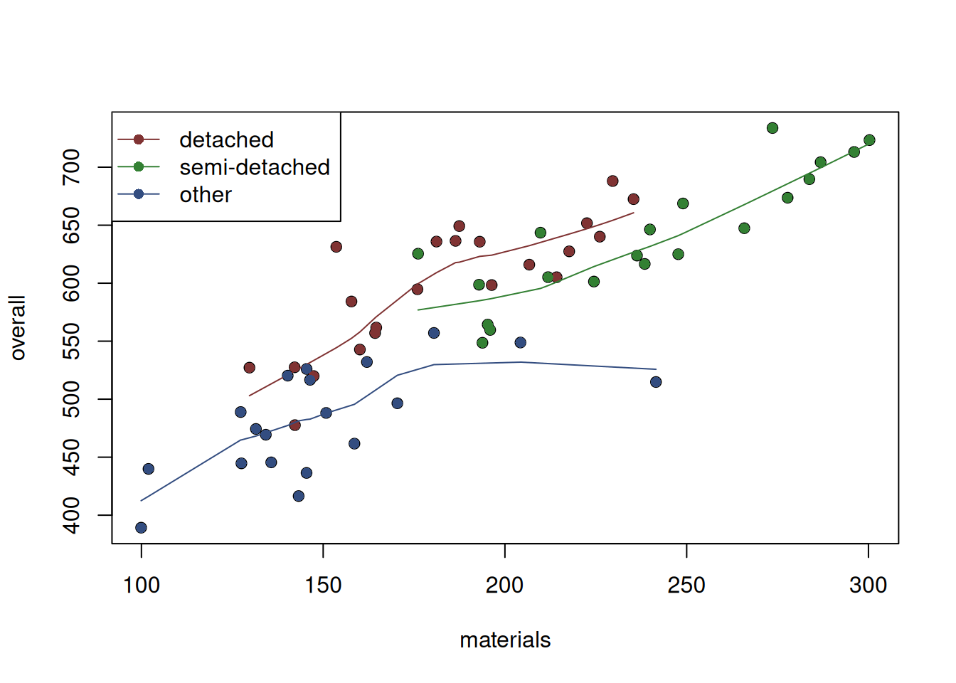
Figure 13.2: Scatterplot of material vs overall costs for the three property types.
It is hard to tell whether the relation changes (i.e. whether the material costs impact the overall costs differently for each of the property types), but it looks like the overall cost of semi-detached properties is higher than detached and other ones. If we were to construct several independent models, we would expect that on average, the semi-detached properties would cost more than the others, which should translate to the higher value of the intercept if we draw the line just through the cloud of the green points. The “other” should have the lowest intercept, because the points are concentrated at the bottom of the plot. Finally, the “detached” should be somewhere in the middle.
To make this switch more natural, we can introduce the dummy variables in regression model. What we could do in this case is have an intercept for one of the categories (for example, for other) and then have some parameters that would either increase or decrease it depending on the type of the property. Luckily, R can introduce them automatically, and we do not need to do anything additional to make it work. We only need to make sure that the respective categorical variable (type in our case) is encoded as a factor:
## [1] "factor"And then we can add it in the regression model:
costsModelWithType <- alm(overall~size+materials+projects+year+type,
                          SBA_Chapter_11_Costs, loss="MSE")
What R does in this case is expands the categorical variable in a set of dummies and uses the first level as a baseline, dropping it from the model (we’ll discuss why in a moment). In our data, this level is “detached”:
## [1] "detached" "semi-detached" "other"The summary of the produced model shows the values of the parameters for each of the levels of type:
## Response variable: overall
## Distribution used in the estimation: Normal
## Loss function used in estimation: MSE
## Coefficients:
##                     Estimate Std. Error Lower 2.5% Upper 97.5%
## (Intercept)       -3231.6672  3204.3686 -9656.0394   3192.7050
## size                  1.0202     0.5876    -0.1578      2.1982
## materials             0.8388     0.2264     0.3850      1.2926 *
## projects             -5.6514     2.8166   -11.2984     -0.0044 *
## year                  1.7984     1.5971    -1.4037      5.0004
## typesemi-detached   -39.6631    13.3095   -66.3471    -12.9791 *
## typeother           -76.4043    11.2599   -98.9791    -53.8295 *
##
## Error standard deviation: 31.3843
## Sample size: 61
## Number of estimated parameters: 7
## Number of degrees of freedom: 54
## Information criteria:
##      AIC     AICc      BIC     BICc
## 602.1246 604.8938 619.0116 624.7036
Each of the parameters for the variables typesemi-detached and typeother show how the intercept will change in comparison with the baseline category (detached in our case) if we have this type of property, i.e. whether the line will be above or below the line for the detached properties and by how much.
To understand this clearer, consider the example where we have a type="detached" property. In that case, the dummy variables typesemi-detached and typeother both would be equal to zero, which means that the respective parameters in the output above will be ignored. As a result, the intercept for that line would be -3231.6672. On the other hand, if we have the semi-detached property, the intercept will be -3231.6672 -39.6631= -3271.3303.
Now, why does R drop one of the levels? The simple explanation is that if we have those three dummy variables in the house_types variable, one of them can be considered redundant, because if we know that the property is neither detached, nor semi-detached, then it must be “other”. See example of the fifth project:
##      typedetached typesemi-detached         typeother
##                 0                 0                 1
So, having all levels is simply unnecessary. But there is a mathematical explanation as well. It relates to the so called “dummy variables trap”.
13.1.1 Dummy variables trap
Consider a regression model without the dummy variables that we previously estimated in Section 11.1:
costsModel01 <- alm(overall~size+materials+projects+year,
                    SBA_Chapter_11_Costs, loss="MSE")
summary(costsModel01)
## Response variable: overall
## Distribution used in the estimation: Normal
## Loss function used in estimation: MSE
## Coefficients:
## Estimate Std. Error Lower 2.5% Upper 97.5%
## (Intercept) 614.3227 4337.3590 -8074.4514 9303.0968
## size 1.3471 0.6989 -0.0529 2.7471
## materials 0.8706 0.3112 0.2473 1.4939 *
## projects -1.5921 3.7971 -9.1986 6.0144
## year -0.1602 2.1621 -4.4915 4.1711
##
## Error standard deviation: 43.4158
## Sample size: 61
## Number of estimated parameters: 5
## Number of degrees of freedom: 56
## Information criteria:
## AIC AICc BIC BICc
## 639.9341 641.4896 652.5993 655.7967As discussed in Section 11.4, this model can be written as: \[\begin{equation} overall_j = 614.3227 + 1.3471 size_j + 0.8706 materials_j - 1.5921 projects_j - 0.1602 year_j + \epsilon_j . \tag{13.1} \end{equation}\] We can notice in the formula above, that we have a variable right after each of the parameters. In fact, the intercept can also be represented in the same form, the main difference is that it is multiplied by 1 instead of anything else: \(614.3227 = 614.3227 \times 1\).
Now if we add all the three dummy variables in the model, for each specific observation, we will have an issue called “perfect multicollinearity” (we will discuss it in more detail in Section 15.3.1), where the included variables are linearly related and lead to estimation issues in the model. In our case, we can say that the sum of the three dummy variables for any specific observation equals to one (which is that latent variable for the intercept that we mentioned above). So, by including all of them in the model together with the intercept, we will not be able to distinguish the specific effect of one variable on the response variable from the other one. Having the linear combination detached + semi-detached + other = 1, the estimates of the intercept and the three parameters for the type levels are not uniquely defined and can be anything as long as their combination leads to the line going through the specific segments of points.
To better demonstrate this idea, consider an artificial example of \(sales\) of a product and three dummy variables \(colourRed\), \(colourGreen\) and \(colourBlue\), which are just three categories of a \(colour\) of the product. The three dummy variables form the relation shown in the scatterplot in Figure 13.3.
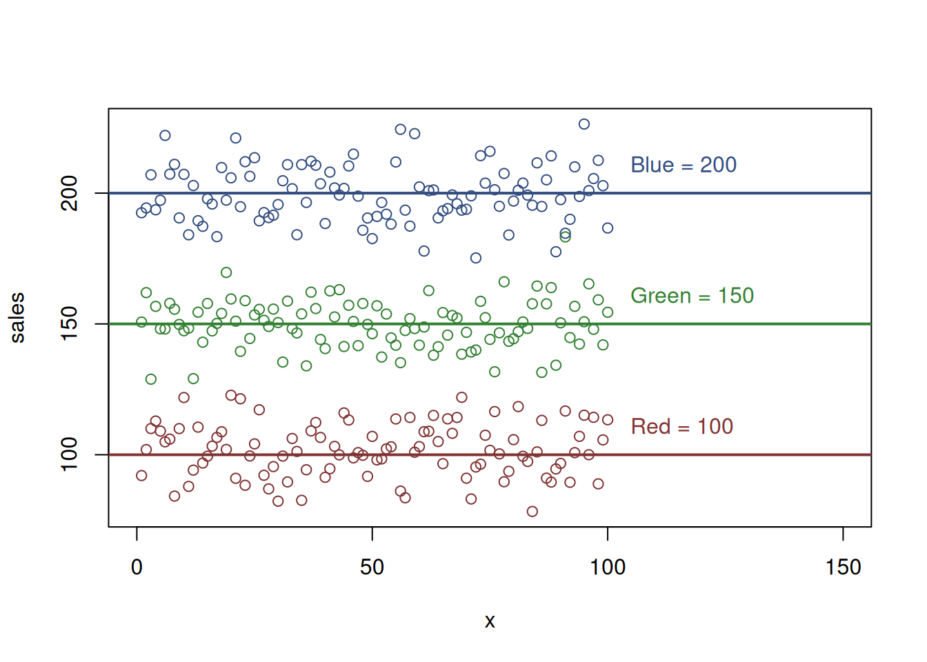
Figure 13.3: Artificial example with sales and colours
The horizontal lines in Figure 13.3 show the average sales of products of each colour. We have designed this example in a way that the sales of the red product are on average 100, the sales of the green one are 150, and for the blue one, they are 200. In reality, we never know these values, and having only the knowledge that there are three colours of product, we need to estimate these parameters.
From the regression perspective, if we include the intercept and the three parameters, we would have four lines to draw instead of three, because the intercept would correspond to a separate one. In that situation, we have infinite combinations of how to draw the lines in this case. For example, the intercept can go through the point zero, and the others would go through 100, 150 and 200 respectively. This corresponds to the situation where we do not include intercept in the model and is shown in Figure 13.3. In that case, the model becomes estimable (we got rid off of one of lines). Alternatively, we could tell the regression to draw the intercept from the same point as in case of the red colour. This situation would then correspond to the one shown in Figure 13.4, and the values of parameters for the red, green and blue would be equal to 0, 50 and 100 respectively because their values are defined relative to the intercept value.
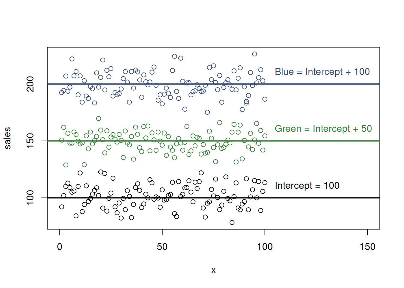
Figure 13.4: Artificial example with sales and colours and one of colours excluded.
In both of these cases, regression would be able to estimate the parameters, because we impose some restrictions that help it. But if we do not do it, the intercept can go anywhere and the parameter for each of colours would not be uniquely defined. An example of this situation is shown in Figure 13.5, where intercept was set to 125, and the rest are defined based on this: -25, 25, and 75 respectively for the red, green and blue colours. But it could also be 124, and the other parameters would be -24, 26 and 76. The number of combinations is infinite and if we do not impose any restrictions and do not help the regression, we will not get any specific answer.
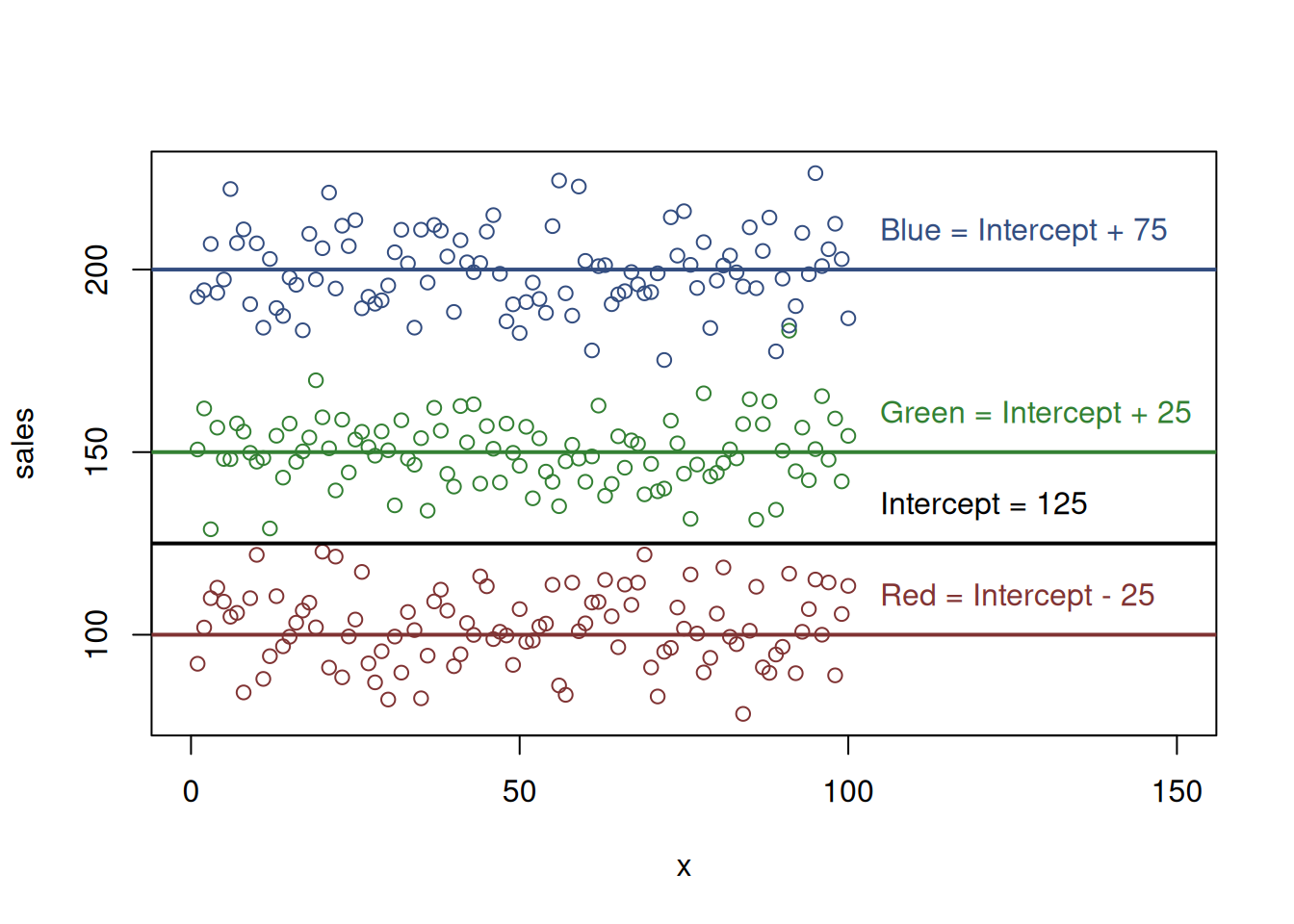
Figure 13.5: Artificial example with sales and colours, dummy variables trap.
To avoid the dummy variables trap, we can either drop one of levels (which is done by R automatically, as described above), or remove the intercept. The latter, however, has some consequences, because the intercept plays an important technical role, characterising where the line intersects the y-axis. If it is dropped, the model will imply that the intersection is happening at the origin (where all variables are equal to zero), and this might cause issues in the quality of a fit (see Section 11.2).
Finally, it is recommended in general not to drop dummy variables one by one, if for some reason you decide that some of them are not helping. If, for example, we decide not to include detached and only have the model with semi-detached, then the meaning of the dummy variables will change - we will not be able to distinguish the detached from other properties. Furthermore, while some dummy variables might not seem important (or significant) in regression, their combination might improve the model, and dropping some of them might be damaging for the model in terms of its predictive power. So, it is more common either to include all levels (but one to avoid the trap) of categorical variable or not to include any of them.
13.1.2 What about the variables in the ordinal scale?
In comparison with the nominal scale, the ordinal one has the “order” property. This means that we can say which of the levels can be placed higher than the others. If we evaluate all the property projects on the scale of “big”, “medium” and “small”, trying to capture the effort needed to construct specific buildings, that would be the ordinal scale. The logic temptation in this case is to assign some numbers to each of the elements of this scale, e.g. 1 for “big”, 2 for “medium” and 3 for “small”. The next step which is taken by some analysts is to include this new variable in regression as is. But there is an important aspect in such decision which needs to be taken into account: the ordinal scale does not have distance. This means that we could also assign 5, 8 and 13 to the specific levels, and we would not loose any original information. So, if you decide to include the variable in the regression model, you need to have very good motivation why the change from “big” to “medium” should have exactly the same effect as the change from “medium” to “small”. Typically, this is not the case, and shifting the assigned numbers to capture such switch is too hard and fruitless. So, in general, you should not include the ordinal variables in the regression model as is, and you need to transform them into a set of dummy variables, similar to how it is done for the nominal scale.