10.5 What about the “Timber Lend” company?
Coming back to the example that motivated this chapter, there is a way we can improve the model for the company and help them in making better decisions. After all, the determination coefficient of the model of volume from height was just 0.358.
First, we check how the relation between the diameter and the volume looks (Figure 10.12)
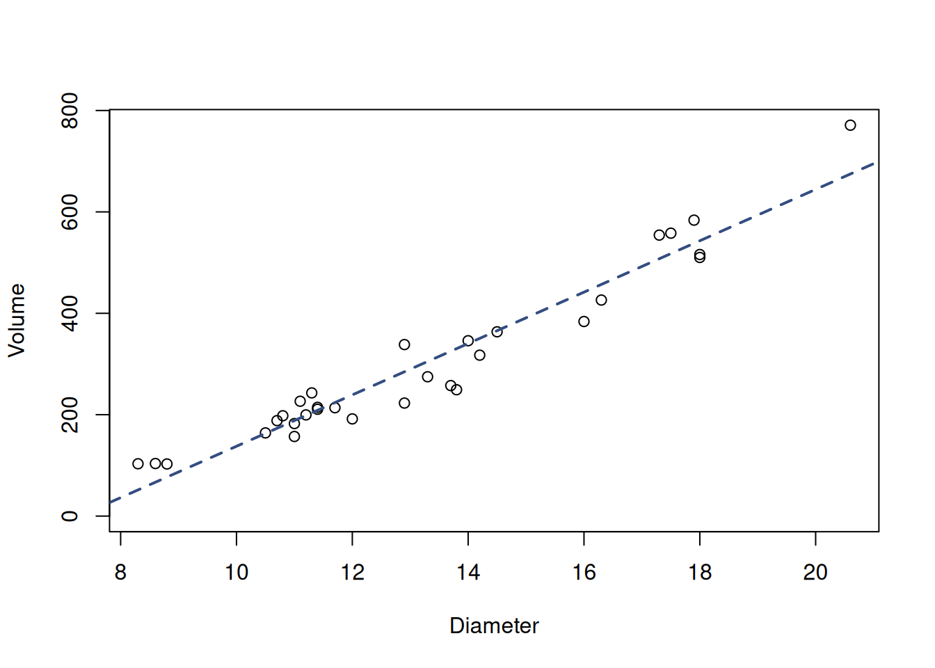
Figure 10.12: Scatterplot matrix of the trees volume and dimeter.
It might not be apparent for an inexperienced analyst, but the relation between the diameter and volume is non-linear, because the points for the lowest and highest diameters lie consistently above the straight line. Even if this relation is not apparent visually, there is a fundamental reason for its existence: trunks of trees have a shape close to cylinder. Some of you might remember from geometry that the volume of a cylinder is calculated as:
\[\begin{equation}
V = h \pi r^2 ,
\tag{10.33}
\end{equation}\]
where \(V\) is the volume, \(h\) is the height, \(r\) is the radius and \(\pi\) is the constant number. The diameters that we have in the data equal to \(d=2 \times r\). Having this fundamental formula, implies that the relation between the diameter and volume should be indeed non-linear. Based on that, we can create a new variable, which could be called cylinder:
Furthermore, because trunks of trees are not exactly cylinders, our model can be represented as: \[\begin{equation*} volume = \beta_0 + \beta_1 cylinder + \epsilon_j. \end{equation*}\]
This model in R gives is much more reasonable than either the model of volume from height or volume from diameter. We can fit it and see how much variability it explains:
# Fit the model
slmTreesCyl <- lm(volume~cylinder, SBA_Chapter_10_Trees)
# Get the number of observations
n <- nobs(slmTreesCyl)
# Calculate R^2
1 - sum(resid(slmTreesCyl)^2) / (var(actuals(slmTreesCyl))*(n-1))
## [1] 0.9777898Remark. While in general, we should not compare models based on R\(^2\), in this specific case we can because the number of explanatory variables in the two models is exactly the same.
As we see the model of volume from cylinders explains the data much better than the previous one.
In the formula of the cylinder (10.33), we do not have any error term. Why do we expect it to be in the model that we fit? Shouldn’t R\(^2\) be equal to one in our example?
We do not expect to have zero error in this case, because the trunks of trees are not perfect cylinders: the diameter at the top of the tree is smaller than the diameter at the bottom, and trees have some curvature, deviating in shape from the perfect cylinder. Due to these factors, the formula (10.33) does not perfectly describe the volume of the tree, but instead is a good approximation of it.
As for the coefficients of the model, based on our sample, they were:
## (Intercept)    cylinder
## -2.43730518  0.02124751
Using some specific measurements of a tree, we can get its expected volume. For example, if a tree has the height of 80 and diameter of 10.7, our new variable cylinder would be \(80 \times 11.1^2 = 9856.8\). Inserting this value in the equation, we get the expected volume:
\[\begin{equation*} volume = -2.44 + 0.02 \times 9856.8 \approx 207.00 , \end{equation*}\] which is not too far from the real volume of 226.5 that we have in the data (observation number 9). While this is not a perfect estimate of volume, it allows improving the operational process for the “Timber Lend” company, hopefully reducing some costs.