6.5 Confidence interval
As mentioned in Section 1.4, we always work with samples and inevitably we deal with randomness just because of that even, when there are no other sources of uncertainty in the data. For example, if we want to estimate the mean of a variable based on the observed data, the value we get will differ from one sample to another. This should have become apparent from the examples we discussed earlier. And, if the LLN and CLT hold, then we know that the estimate of our parameter will have its own distribution and will converge to the population value with the increase of the sample size. This is the basis for the confidence and prediction interval construction, discussed in this section. Depending on our needs, we can focus on the uncertainty of either the estimate of a parameter, or the random variable \(y\) itself. When dealing with the former, we typically work with the confidence interval - the interval constructed for the estimate of a parameter, while in the latter case we are interested in the prediction interval - the interval constructed for the random variable \(y\).
In order to simplify further discussion in this section, we will take the population mean and its in-sample estimate as an example. In this case we have:
- A random variable \(y\), which is assumed to follow some distribution with finite mean \(\mu\) and variance \(\sigma^2\);
- A sample of size \(n\) from the population of \(y\);
- Estimates of mean \(\hat{\mu}=\bar{y}\) and variance \(\hat{\sigma}^2 = s^2\), obtained based on the sample of size \(n\).
What we want to get by doing this is an idea about the population mean \(\mu\). The value \(\bar{y}\) does not tell us much on its own due to randomness and if we do not capture its uncertainty, we will not know, where the true value \(\mu\) can be. But using LLN and CLT, we know that the sample mean should converge to the true one and should follow normal distribution. So, the distribution of the sample mean would look like this (Figure 6.15).
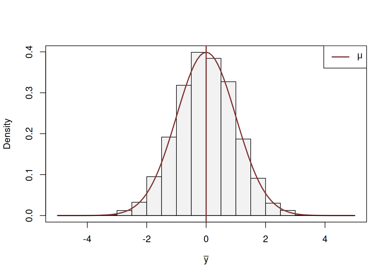
Figure 6.15: Distribution of the sample mean.
On its own, this distribution just tells us that the variable is random around the true mean \(\mu\) and that its density function has a bell-like shape. In order to make this more useful, we can construct the confidence interval for it, which would tell us where the true parameter is most likely to lie. We can cut the tails of this distribution to determine the width of the interval, expecting it to cover \((1-\alpha)\times 100\)% of cases. In the ideal world, asymptotically, the confidence interval will be constructed based on the true value, like this:
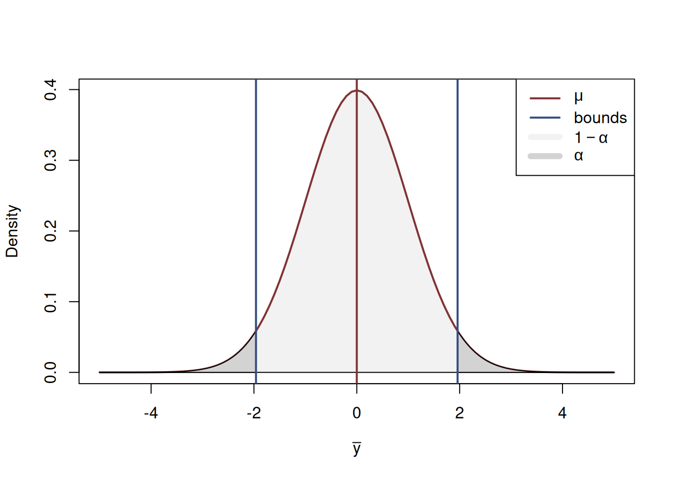
Figure 6.16: Distribution of the sample mean and the confidence interval based on the population data.
Figure 6.16 shows the classical normal distribution curve around the population mean \(\mu\), confidence interval of the level \(1-\alpha\) and the cut off tails, the overall surface of which corresponds to \(\alpha\). The value \(1-\alpha\) is called confidence level, while \(\alpha\) is the significance level. By constructing the interval this way, we expect that in the \((1-\alpha)\times 100\)% of cases the value will be inside the bounds, and in \(\alpha\times 100\)% it will not.
In reality we do not know the true mean \(\mu\), so we do a slightly different thing: we construct a confidence interval based on the sample mean \(\bar{y}\) and sample variance \(s^2\), hoping that due to LLN (Section 6.2) they will converge to the true values. We use Normal distribution, because we expect CLT (Section 6.3) to work. This process looks something like in Figure 6.17, with the bell curve in the background representing the true distribution for the sample mean and the curve on the foreground representing the assumed distribution based on our sample:
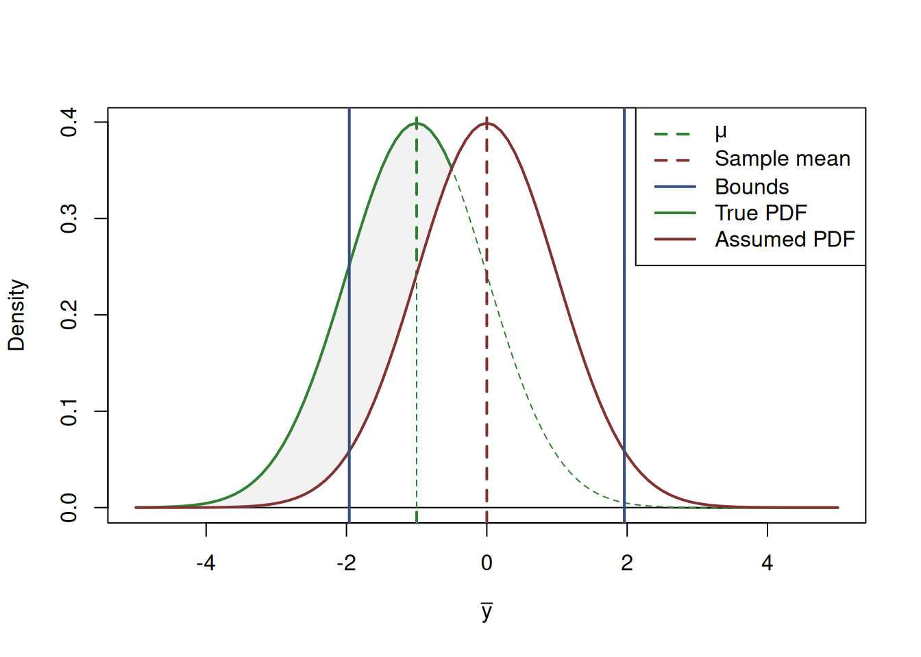
Figure 6.17: Distribution of the sample mean and the confidence interval based on a sample.
So, what the confidence interval does in reality is tries to cover the unknown population mean, based on the sample values of \(\bar{y}\) and \(s^2\). If we construct the confidence interval of the width \(1-\alpha\) (e.g. 0.95) for thousands of random samples (thousands of trials), then in \((1-\alpha)\times 100\)% of cases (e.g. 95%) the true mean will be covered by the interval, while in \(\alpha \times 100\)% cases it will not be. The interval itself is random, and we rely on LLN and CLT, when constructing it, expecting for it to work asymptotically, with the increase of the number of trials.
Another way to think about the confidence interval is that it shows the variability of the estimate of the parameter from one sample to another. In the ideal situation of the estimate being consistent and unbiased (Section 6.4), the true value of parameter will be covered by the interval in \((1-\alpha)\times 100\)% of cases. If the estimator produces unreliable results, the interval will only show how the estimate changes on average if we change the sample.
Mathematically the red bounds in Figure 6.17 are represented using the following well-known formula for the confidence interval: \[\begin{equation} \mu \in (\bar{y} + t_{\alpha/2}(df) s_{\bar{y}}, \bar{y} + t_{1-\alpha/2}(df) s_{\bar{y}}), \tag{6.4} \end{equation}\] where \(t_{\alpha/2}(df)\) is Student’s t-statistics for \(df=n-k\) degrees of freedom (\(n\) is the sample size and \(k\) is the number of estimated parameters, e.g. \(k=1\) in our case) and level \(\alpha/2\), and \(s_{\bar{y}}=\frac{1}{\sqrt{n}}s\) is the estimate of the standard deviation of the sample mean (see proof below). If we knew for some reason the true variance \(\sigma^2\), then we could use z-statistics instead of t, but we typically do not, so we need to take the uncertainty about the variance into account as well, thus the use of t-statistics (see discussion of sample mean tests in Section 8.1).
Proof. We are interested in calculating the variance of \(\bar{y}=\frac{1}{n} \sum_{j=1}^n y_j\). If \(s\) is the standard deviation of the random variable \(y\), then \(\mathrm{V}(y_j) = s^2\). The following derivations assume that \(y_j\) is i.i.d. (specifically, not correlated with each other). \[\begin{equation*} \begin{aligned} \mathrm{V}(\bar{y}) = & \mathrm{V}\left(\frac{1}{n} \sum_{j=1}^n y_j \right) = \frac{1}{n^2} \mathrm{V} \left(\sum_{j=1}^n y_j \right) = \\ & \frac{1}{n^2} \sum_{j=1}^n \mathrm{V} \left( y_j \right) = \frac{1}{n^2} \sum_{j=1}^n s^2 = \\ & \frac{1}{n} s^2 \end{aligned} \end{equation*}\] Based on this, we can conclude that \(s_{\bar{y}}=\sqrt{\mathrm{V}(\bar{y})}= \frac{1}{\sqrt{n}} s\).
Note, that in order to construct confidence interval, we do not care what distribution \(y\) follows, as long as LLN and CLT hold.