4.6 Convolution of distributions
Whenever we want to add or take a mean of two random variable, and want to know what we get a result, we are dealing with the operation called in mathematics “convolution”. By doing convolution we combine two random processes to form a new one.
4.6.1 Convolution of two discrete distributions
To explain it better, we take a step back and consider a case of rolling dices. As we discussed, in that case we are dealing wi the uniform distribution (Section 3.6): it is equally probably to get 1, 2, 3, 4, 5 or 6 when you roll a dice once. Now, what would happen if we roll two dices at the same time?
Let us record the value on one dice as \(x\), and the value on the second one as \(y\). Rolling both of them, means that we need to add \(x\) to \(y\) to get a new score \(z\). For example, we had 3 on one dice and 5 on the other one, which means that \(x=3\), \(y=5\) and \(z=x+y=3+5=8\). The span of values of \(z\) is now between 2 and 12, because the lowest score for each die is 1 (thus \(1+1=2\)), while the highest one is 6 (6+6=12).
But what happens with the probability distribution? Remember, it was uniform for both dices and looked like this (Figure 4.20):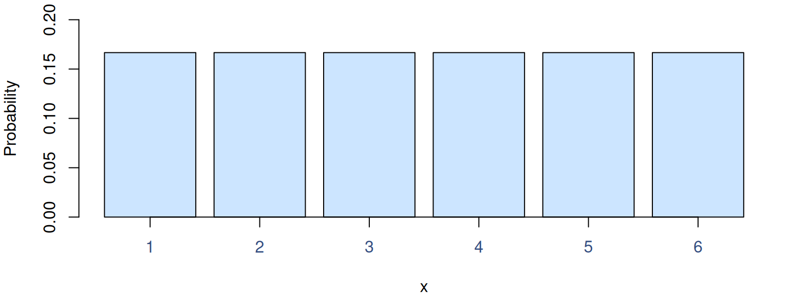
Figure 4.20: Probability Mass Function of Uniform distribution for 1d6.
To get the PMF of the new convolved distribution, we need to assign probabilities for each of the new combined values. Getting the score of 2 is only possible if we have 1 on each dice, which corresponds to the probability of \(\frac{1}{6}\) for each of them, meaning that this can happen only in \(\frac{1}{6} \times \frac{1}{6} = \frac{1}{36}\) cases. The score \(z=3\) is possible if we get either \(x=1\) and \(y=2\) or \(x=2\) and \(y=1\). This translates to the probability of \(\frac{1}{36} + \frac{1}{36} = \frac{2}{36} = \frac{1}{18}\). We could continue with other distributions, obtaining probability of each outcome from \(z=2\) to \(z=12\).
One way of looking at this process, is to first acknowledge that \(y=z-x\) and then by sliding one distribution above the other by changing the value of \(x\). For example, to have \(z=3\) we can have \(x=1\) and \(y=3-1=2\), or \(x=2\) and \(y=3-2=1\). This corresponds to the sliding shown in Figure 4.21, where the red distribution is placed above the blue one and in this specific example, we get an intersection of two bars, each of which gives us the same \(z=3\) (which is shown on the right-hand side plot). The probabilities of each bar are \(\frac{1}{6}\), the intersection gives us the multiplication of those probabilities (thus \(\frac{1}{36}\)) and we have two bars that have these intersections, so the final answer is the same as we obtained above: \(\frac{1}{36} + \frac{1}{36} = \frac{1}{18}\). The barplot on the right-hand side of the image shows how specific probabilities appear. The height of the bars corresponds to the probability of the specific \(z\) score.
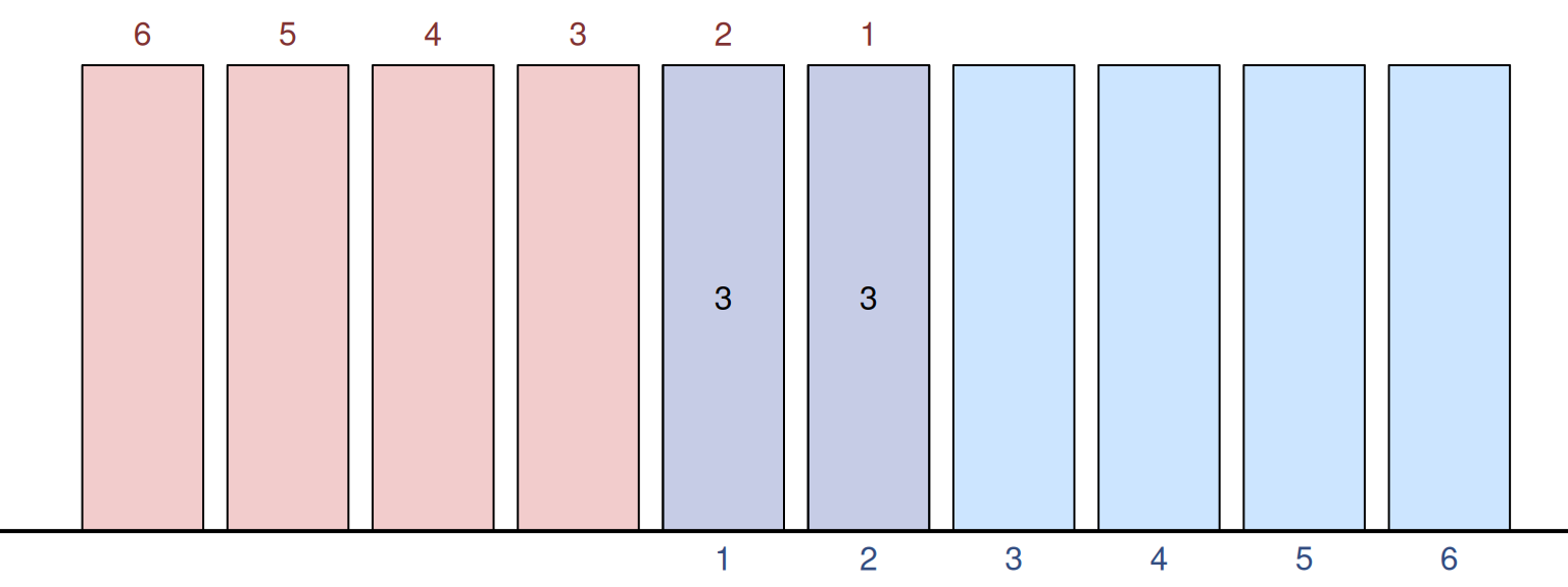
Figure 4.21: Convolution of two PMFs for 1d6, giving the join score of 3.
The more we move the red bars to the right, the more intersections we will have, giving us higher and higher probability of occurrence until we reach the moment shown in Figure 4.22.
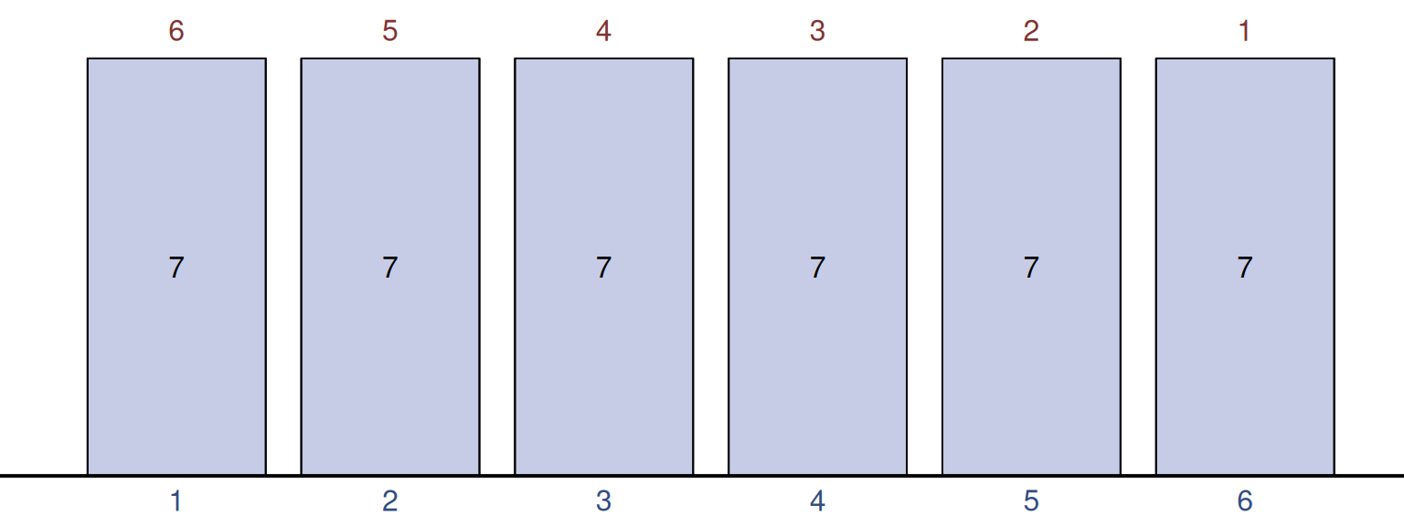
Figure 4.22: Convolution of two PMFs for 1d6, giving the join score of 7.
In this specific example, we can obtain \(z=7\) 6 different ways, which means that the probability of that outcome is \(\frac{1}{36} \times 6 = \frac{1}{6}\). This is the highest probability outcome if you roll two 6 sided dices (2d6). But that’s not all, after that, we can continue sliding the distribution, and we will notice that the probability of outcomes starts declining as well (Figure 4.23), because we have fewer and fewer intersections between the distributions that would give us the specific scores.
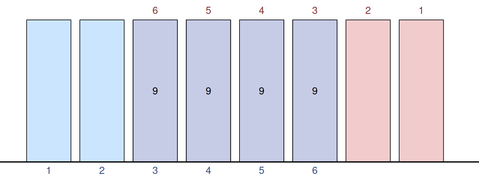
Figure 4.23: Convolution of two PMFs for 1d6, giving the join score of 9.
Collecting all the probabilities after such sliding, we can visualise the PMF of \(z\) (convolution of two uniform distributions), which is shown in Figure 4.24, where we decided not to simplify the ratios for simplicity.
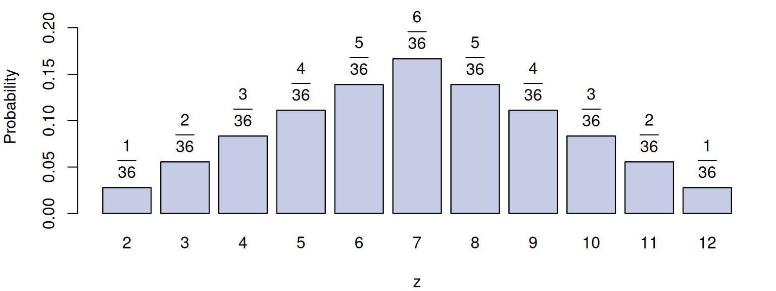
Figure 4.24: Probability Mass Function of the sum of two Uniform distributions for 1d6.
4.6.2 Convolution of two continuous distributions
The logic with convolution of two continuous distributions is similar to the one for the discreet, but instead of adding bars, we need to calculate the sizes of the intersected surfaces. Mathematically, this is done by taking an integral (see details in Subsection 4.6.3).
Visually, this is shown in Figure 4.25 for the sum of two variables following the identical Standard Normal distributions (zero mean and unit variance).
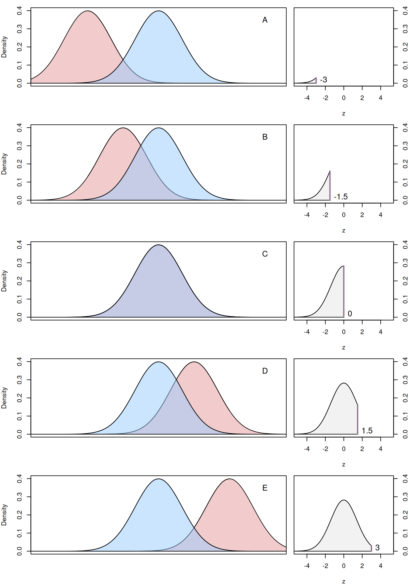
Figure 4.25: Convolution of two standard Normal distributions.
Figure 4.25 shows five special cases of the sliding with the red distribution moving over the blue one. The purple area where distributions intersect corresponds to the probability density for each specific value of \(z=x+y\), which on the right of each plot is shown with a vertical purple line. We can see that this area reaches its maximum when two distributions coincide. This corresponds to the peak in the new distribution.
There is a mathematical proof that a sum of two variables \(x\) and \(y\) following Normal distributions with some means \(\mu_x\) and \(\mu_y\) and variances \(\sigma_x^2\) and \(\sigma_y^2\) is another Normal distribution with \(\mu_z=\mu_x+\mu_y\) and \(\sigma_z^2=\sigma_x^2+\sigma_y^2 + 2 \sigma_{x,y}\), where \(\sigma_{x,y}\) is the covariance between them. If the two distributions are independent, the covariance becomes equal to zero. If the two distributions are identical (as in Figure 4.25) with zero means and unit variances, the resulting distribution will be \(\mathcal{N}(0, 2)\), which we can see in the right-hand sides of the image.
So far, we looked at the convolution of the symmetric distributions. But the situation would be a bit different for the asymmetric ones, because in reality the distribution that we slide over needs to be flipped vertically to reflect the idea we discussed in case of the convolution of discrete distributions in Subsection 4.6.1: there is a multitude of values of \(x\) and \(y\) that give a specific value of \(z\). For the continuous distribution, for example, the number \(z=4\) can be achieved by \(x=2\) and \(y=2\), by \(x=2.1\), \(y=1.9\), by \(x=2.0000001\) and \(y=1.9999999\), by \(x=10\), \(y=-6\), etc - the number of possible combinations is infinite. But not all of them are equally possible, which is reflected by the PDFs of \(x\) and \(y\).
To see the idea of flipping clearer, consider two Exponential distributions (discussed in Section 4.5) with \(\lambda=1\). Three specific points during the sliding would look like those shown in Figure 4.26. They correspond to situations when \(z=1\), \(z=3\) and \(z=5\).
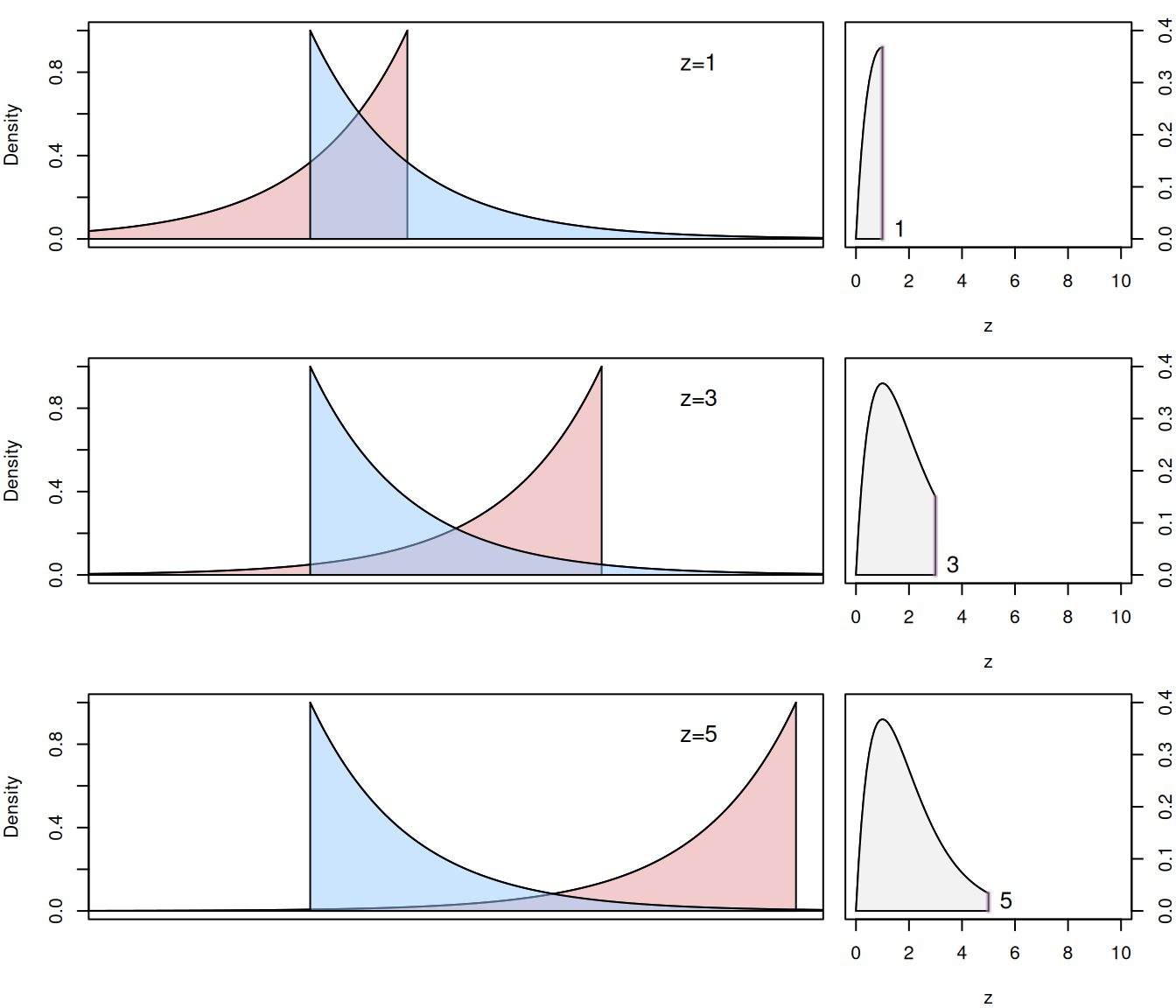
Figure 4.26: Convolution of two Exponential distributions with \(\lambda=1\).
For that case, the resulting distribution would not be symmetric. It would have values starting from zero (because there is no intersection between the red and the blue areas for negative values), have a long right tail and a hump, not too far from zero.
Similar mechanism is used for convolutions of other distributions. The interesting point, which we will come back to in Chapter 6, is that if many identical distributions are convolved (so we take sum of many random variables that follow those distributions), the resulting distribution would be Normal. In the examples in this Chapter, this becomes apparent even with the uniform distribution: if we convolve the distribution \(z\) with another discrete uniform distribution, the resulting one would be symmetric and it would start looking closer and closer to the Normal distribution. This, for example, means, that if you roll 30 6-sided dice, the distribution of the outcome could be approximated by the Normal one.
4.6.3 Mathematics behind convolutions
If we have two random variables \(x\) and \(y\) following continuous distributions \(f(x)\) and \(g(y)\) respectively, their sum \(z=x+y\) (convolution) would follow a distribution with PDF \(h(z)\), which can be written as: \[\begin{equation} h(z) = (f * g)(z) := \int_{-\infty}^{\infty} f(x) g(z-x) dx . \tag{4.21} \end{equation}\] The sliding that we discussed in the previous subsections, in this formula is done by the element \(g(z-x)\), which takes values from the right tail of distribution due to \(z-x\), thus reflecting the idea that we can obtain the same value of \(z\) with a set of combinations of \(x\) and \(y\), each having some assigned density value from the functions \(f(x)\) and \(g(y)\) respectively.