4.2 Continuous Uniform distribution
Consider an example with elevator. You press the button to call it, and it arrives after some time. This time of arrival can be 0 seconds if the elevator is at your floor, or 1 minute if it is already moving and delivering people to a different floor. From our perspective, we do not know what the state of the elevator is, and we consider each of the possible scenarios equally probable. So, the elevator arriving in 0 seconds has the same probability as it arriving in 5, 15, 30, 55 or 60 seconds. In this case, we could use the continuous uniform distribution to model the lift arrival and to understand, for example, how much time we would need to wait on average.
The contiunuous uniform distribution has similarities to the discrete one, which was discussed in Section 3.6, but due to the different nature of the random variable is parameterised differently. First, because we are discussing continuous variable, it is always defined on a segment of values, from \(a\) to \(b\). For example, we can have a random variable which can take any value from 0 to 10 with equal likelihood. Mathematically, the PDF of continuous distribution can be written as: \[\begin{equation} f(y, a, b) = \left\{\begin{aligned} & \frac{1}{b-a} & \text{ for } y \in [a, b] \\ & 0 & \text{ otherwise } \end{aligned} \right. , \tag{4.1} \end{equation}\] or in a short form \(y \sim \mathcal{U}(a,b)\). It can be represented visually as shown in Figure 4.6.
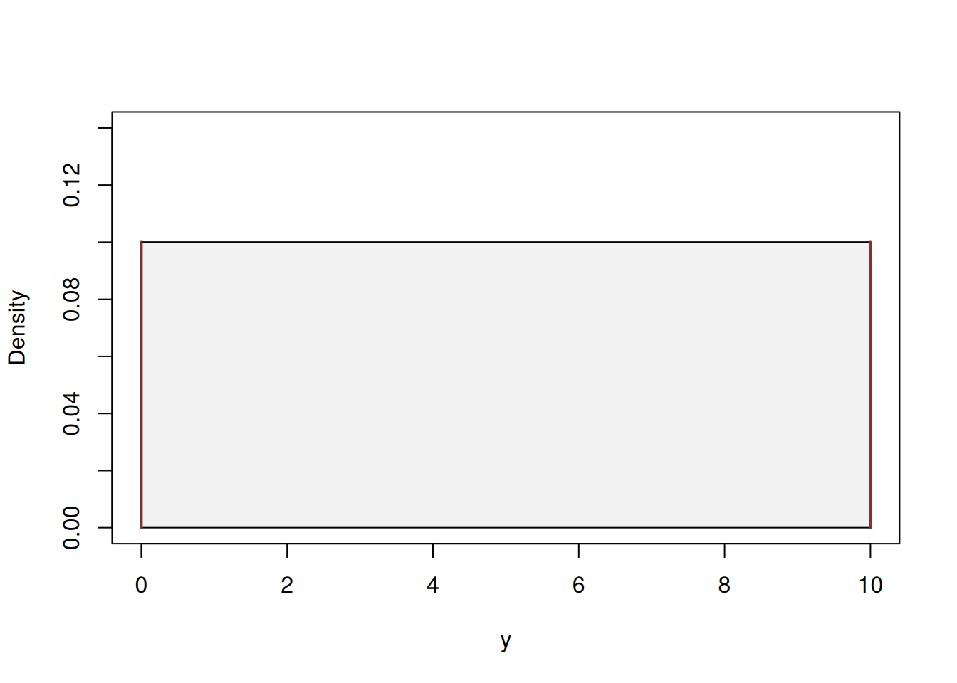
Figure 4.6: Probability Density Function of Continuous Uniform distribution.
According to this distribution, it is equally likely to have 1, 1.1, 1.0001, 9 etc values. The mean of this distribution coincides with the middle of the segment and can be calculated as: \[\begin{equation} \mathrm{E}(y) = \frac{1}{2}(a+b) , \tag{4.2} \end{equation}\] while the variance is calculated as: \[\begin{equation} \mathrm{V}(y) = \frac{1}{12}(b-a)^2 . \tag{4.3} \end{equation}\] The CDF of the Uniform distribution corresponds to the straight line going from the point (a,0) to the point (b,1), as shown in Figure 4.7.
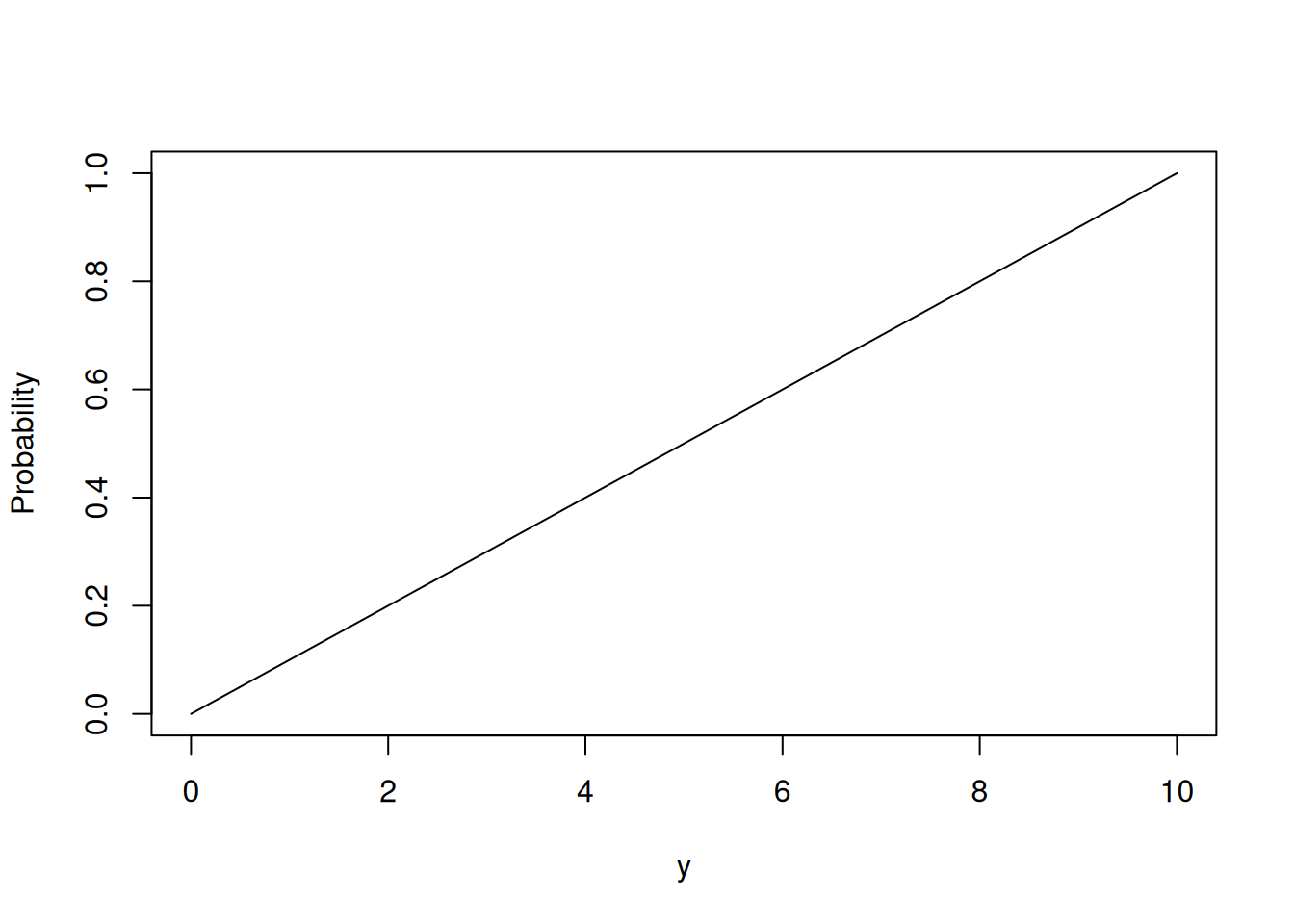
Figure 4.7: Cumulative Density Function of Continuous Uniform distribution.
Mathematically, the CDF can be represented as: \[\begin{equation} F(y, a, b) = \left\{\begin{aligned} & 0 & \text{ if } y<a \\ & \frac{y-a}{b-a} & \text{ for } y \in [a, b] \\ & 1 & \text{ if } y>b \end{aligned} \right. . \tag{4.4} \end{equation}\]
Continuous uniform distribution is sometimes used in statistics as a prior, when a researcher does not have grounds to assume any other, more complicated distribution.
In R, this distribution is implemented in stats package with functions dunif(), punif(), qunif() and runif() for PDF, CDF, QF and random generator respectively.