Chapter 12 Uncertainty in regression
Coming back to the example of real estate costs from Chapter 11, consider a simple linear regression of material vs overall costs, fit to a sub-sample of data. If we fit the line to the first 25 observations we would get a different model than when fitting it to the sample of 50 observations. Figure 12.1 depicts these two situations, where the blue dashed red line corresponds to the bigger sample (fit to the empty red circles in the plot), while the blue solid line represents the model for the smaller sample (blue solid circles).
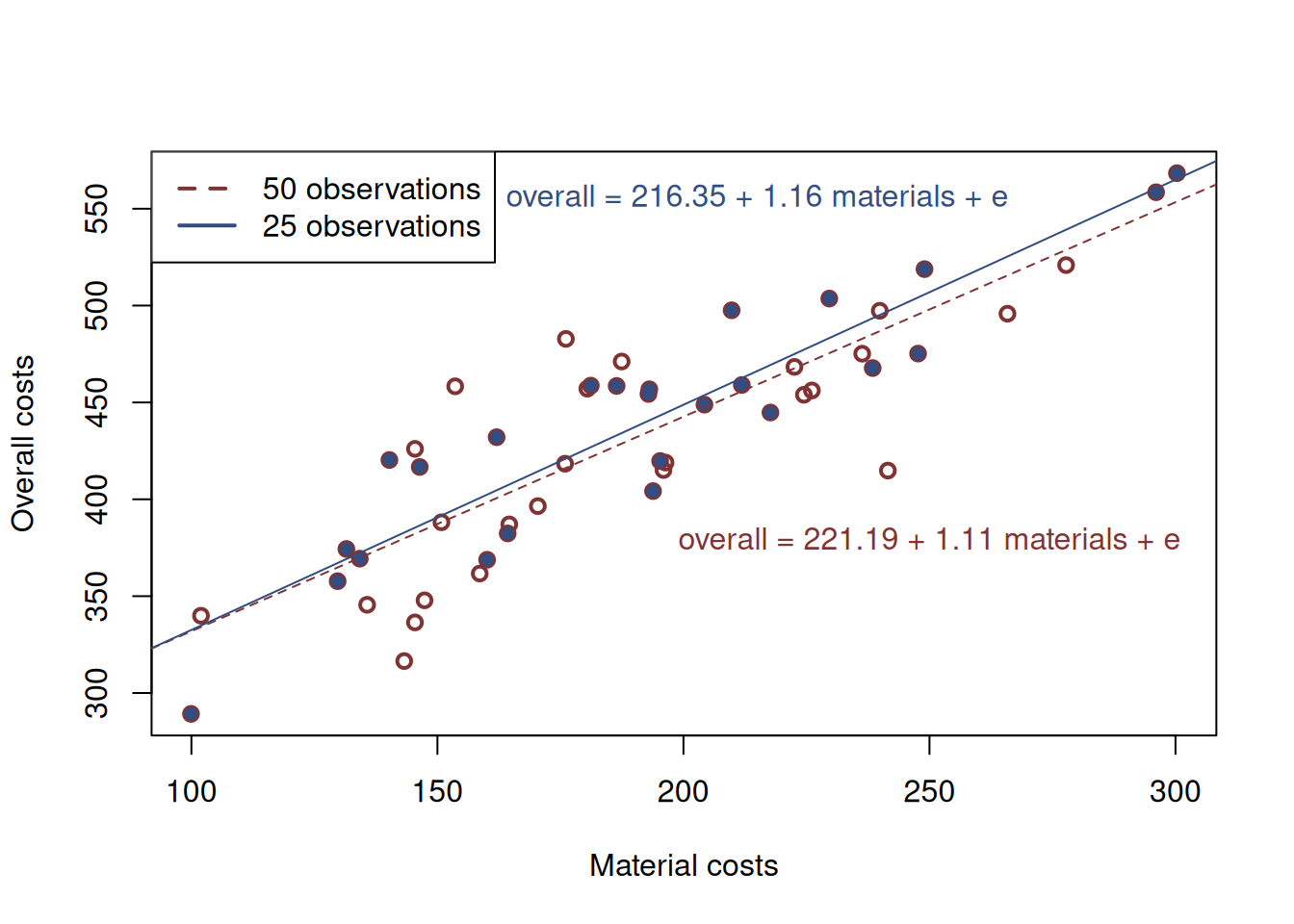
Figure 12.1: Material vs overall costs and two regression lines.
We see that the two lines differ both in terms of their intercepts and their slopes. So, which one of them is correct?
The general view of a spherical statistician in vacuum is that the larger the sample is, the better the model is. While this is correct in general, we would argue that none of the two models is correct. This is because they are both just estimates of the true model (Section 1.1.1 on a sample of data and they both inevitably inherit the uncertainty of the data. This means that whatever regression model we estimate on a sample of data, it will always be incorrect in the sense that it can only be considered as an approximation of the truth.
More importantly, the line will always change when the model is fit to the new sample of data, even if we add only one observation. This is because on different samples, we get different estimates of parameters, which comes from one of the fundamental sources of uncertainty (the second one discussed in Section 1.4). This means that the estimates of parameters are random and might have some distribution of their own.
Exactly the same effect will be observed if we collect a different random sample from the same population, for example, if we worked for a different company that does similar business and collects the same data. In that case, the parameters would be random again, having some sort of a distribution.
To see this point clearer, we fit the same simple regression model to randomly selected subsamples of the original dataset many times and collect the estimates of parameters to plot histograms and see their distribution. This empirical way of capturing uncertainty is called “bootstrap” and we will discuss it in more detail in Chapter ??. The R code below shows how this can be done using the coefbootstrap() function from the greybox package (which implements a simple “Case Resampling” technique):
# Fit the model
costsModelMLR <- alm(overall~materials+size+projects+year, data=SBA_Chapter_11_Costs, loss="MSE")
# Set random seed for reproducibility
set.seed(41)
costsModelMLRBootstrap <- coefbootstrap(costsModelMLR)
Based on that we can plot the histograms of the estimates of parameters as shown in Figure 12.2.
par(mfcol=c(1,2))
# First histogram
hist(costsModelMLRBootstrap$coefficients[,1],
     xlab="Intercept", main="", col=17)
# The estimated coefficient
abline(v=coef(costsModelMLR)[1], col=2, lwd=2)
# Second histogram
hist(costsModelMLRBootstrap$coefficients[,2],
     xlab="Material costs", main="", col=17)
# The estimated coefficient
abline(v=coef(costsModelMLR)[2], col=2, lwd=2)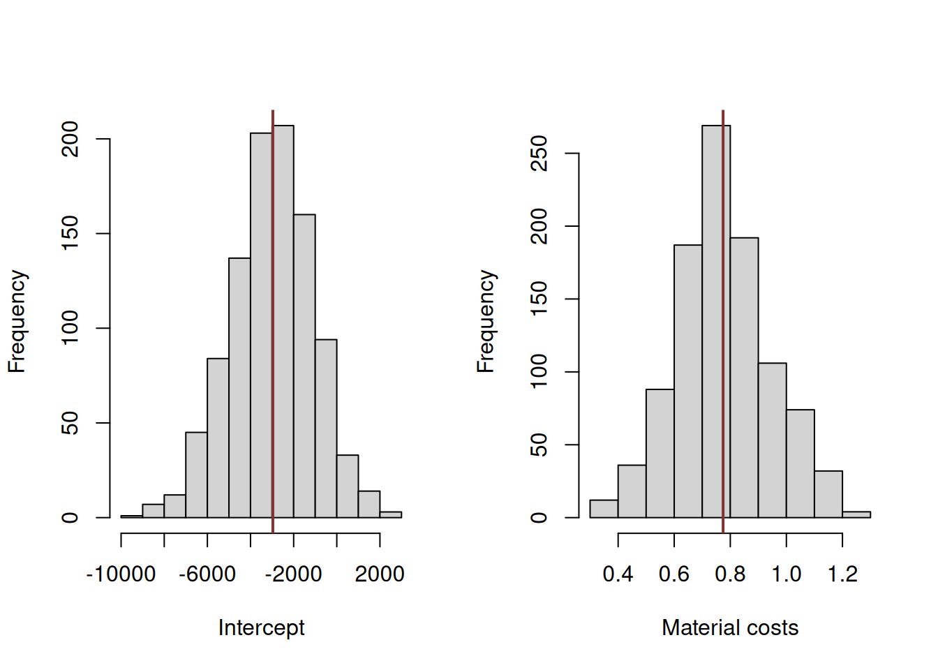
Figure 12.2: Distribution of bootstrapped parameters of a regression model
Figure 12.2 shows the uncertainty around the estimates of parameters. These distributions look similar to the normal distribution and demonstrate the variability of the estimates around the specific values. The vertical lines on the plots show the estimated values of parameters, which hopefully should be close to the ones in the true model. If we were we to repeat this experiment thousands of times, the distribution of estimates of parameters would indeed follow the normal one due to CLT (if the assumptions hold, see Sections 6.3 and Chapter 15).
This example demonstrates that any model applied to the data will always have inherited uncertainty, which should be taken into account. In decision making, you should not rely on just a number from your model, and you should get a general understanding of what the variability about the estimates of parameters is. This has its implications for both parameters analysis and forecasting.