9.2 Ordinal scale
As discussed in Section 1.2, ordinal scale has more flexibility than the nominal one - its values have natural ordering, which can be used, when we want to measure relations between several variables in ordinal scale. Yes, we can use Cramer’s V and \(\chi^2\) test, but this way we would not be using all advantages of the scale. So, what can we use in this case? There are three popular measures of association for variables in ordinal scale:
- Goodman-Kruskal’s \(\gamma\),
- Yule’s Q,
- Kendall’s \(\tau\).
Given that the ordinal scale does not have distances, the only thing we can do is to compare values of variables between different observations and say, whether one is greater than, less than or equal to another. What can be done with two variables in ordinal scale is the comparison of the values of those variables for a couple respondents. Based on that the pairs of the observations can be called:
- Concordant if both \(x_1 < x_2\) and \(y_1 < y_2\) or \(x_1 > x_2\) and \(y_1 > y_2\) - implying that there is an agreement in order between the two variables (e.g. with a switch from a younger age group to the older one, the size of the T-shirt will switch from S to M);
- Discordant if for \(x_1 < x_2\) and \(y_1 > y_2\) or for \(x_1 > x_2\) and \(y_1 < y_2\) - implying that there is a disagreement in the order of the two variables (e.g. with a switch from a younger age group to the older one, the satisfaction from drinking Coca-Cola will switch to the lower level);
- Ties if both \(x_1 = x_2\) and \(y_1 = y_2\);
- Neither otherwise (e.g. when \(x_1 = x_2\) and \(y_1 < y_2\)).
All the measures of association for the variables in ordinal scale rely on the number of concordant, discordant variables and number of ties. All of these measures lie in the region of [-1, 1].
Goodman-Kruskal’s \(\gamma\) is calculated using the following formula: \[\begin{equation} \gamma = \frac{n_c - n_d}{n_c + n_d}, \tag{9.4} \end{equation}\] where \(n_c\) is the number of concordant pairs, \(n_d\) is the number of discordant pairs. This is a very simple measure of association, but it only works with scales of the same size (e.g. 5 options in one variable and 5 options in the other one) and ignores the ties.
In order to demonstrate this measure in action, we will create two artificial variables in ordinal scale:
- Age of a person: young, adult and elderly;
- Size of t-shirt they wear: S, M or L.
Here how we can do that in R:
age <- c(1:3) %*% rmultinom(nrow(mtcars), 1,
                               c(0.4,0.5,0.6))
age <- factor(age, levels=c(1:3),
                 labels=c("young","adult","elderly"))
size <- c(1:3) %*% rmultinom(nrow(mtcars), 1,
                               c(0.3,0.5,0.7))
size <- factor(size, levels=c(1:3),
                 labels=c("S","M","L"))
And here is how the relation between these two artificial variables looks:
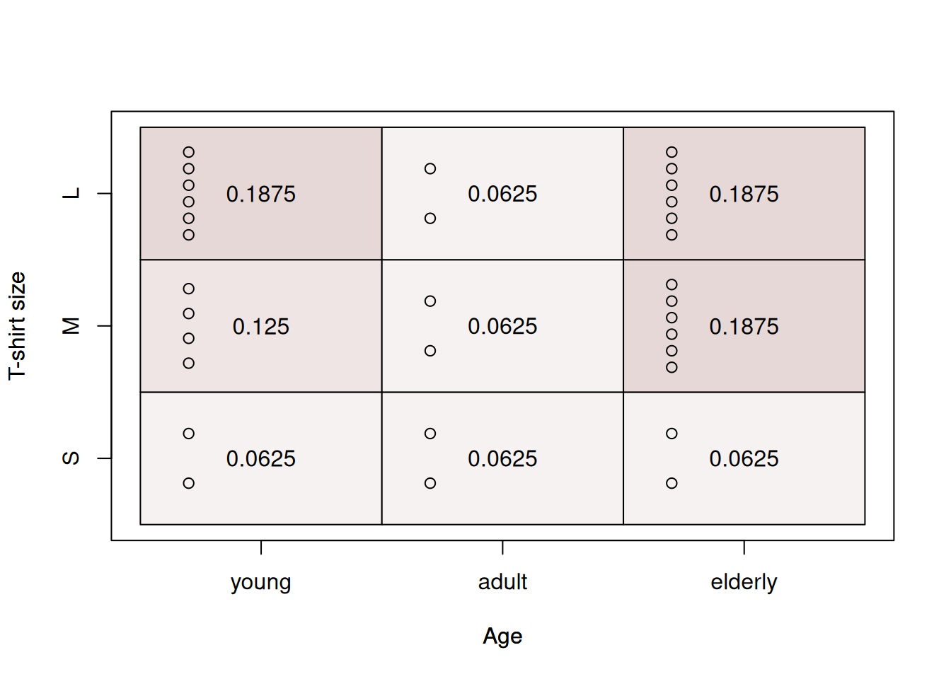
Figure 9.1: Heat map for age of a respondent and the size of their t-shirt.
The graphical analysis based on Figure 9.1 does not provide a clear information about the relation between the two variables. But this is where the Goodman-Kruskal’s \(\gamma\) becomes useful. We will use GoodmanKruskalGamma() function from DescTools package for R for this:
##       gamma      lwr.ci      upr.ci
## -0.03846154 -0.51302449  0.43610141
This function returns three values: the \(\gamma\), which is close to zero in our case, implying that there is no relation between the variables, lower and upper bounds of the 95% confidence interval. Note that the interval shows us how big the uncertainty about the parameter is: the true value in the population can be anywhere between -0.51 and 0.44. But based on all these values we can conclude that we do not see any relation between the variables in our sample.
The next measure is called Yule’s Q and is considered as a special case of Goodman-Kruskal’s \(\gamma\) for the variables that only have 2 options. It is calculated based on the resulting contingency \(2\times 2\) table and has some similarities with the contingency coefficient \(\phi\): \[\begin{equation} \mathrm{Q} = \frac{n_{1,1} n_{2,2} - n_{1,2} n_{2,1}}{n_{1,1} n_{2,2} + n_{1,2} n_{2,1}} . \tag{9.5} \end{equation}\] The main difference from the contingency coefficient is that it assumes that the data has ordering, it implicitly relies on the number of concordant (on the diagonal) and discordant (on the off diagonal) pairs. In our case we could calculate it if we had two simplified variables based on age and size (in real life we would need to recode them to “young”, “older” and “S”, “Bigger than S” respectively):
##        size
## age     S M
##   young 2 4
## adult 2 2## [1] -0.3333333In our toy example, the measure shows that there is a weak negative relation between the trimmed age and size variables. We do not make any conclusions based on this, because this is not meaningful and is shown here just for purposes of demonstration.
Finally, there is Kendall’s \(\tau\). In fact, there are three different coefficients, which have the same name, so in the literature they are known as \(\tau_a\), \(\tau_b\) and \(\tau_c\).
\(\tau_a\) coefficient is calculated using the formula: \[\begin{equation} \tau_a = \frac{n_c - n_d}{\frac{T (T-1)}{2}}, \tag{9.6} \end{equation}\] where \(T\) is the number of observations, and thus in the denominator, we have the number of all the pairs in the data. In theory this coefficient should lie between -1 and 1, but it does not solve the problem with ties, so typically it will not reach the boundary values and will say that the relation is weaker than it really is. Similar to Goodman-Kruskal’s \(\gamma\), it can only be applied to the variables that have the same number of levels (same sizes of scales). In order to resolve some of these issues, \(\tau_b\) was developed: \[\begin{equation} \tau_b = \frac{n_c - n_d}{\sqrt{\left(\frac{T (T-1)}{2} - n_x\right)\left(\frac{T (T-1)}{2} - n_y\right)}}, \tag{9.7} \end{equation}\] where \(n_x\) and \(n_y\) are the number of ties calculated for both variables. This coefficient resolves the problem with ties and can now reach the boundary values in practice. However, this coefficient does not resolve the issue with different scale sizes. And in order to address this problem, we have \(\tau_c\) (Stuart-Kendall’s \(\tau_c\)): \[\begin{equation} \tau_c = \frac{n_c - n_d}{\frac{n^2}{2}\frac{\min(r, c)-1}{\min(r, c)}}, \tag{9.8} \end{equation}\] where \(r\) is the number of rows and \(c\) is the number of columns. This coefficient works for variables with different lengths of scales (e.g. age with 5 options and t-shirt size with 7 options). But now we are back to the problem with the ties…
In R, the cor() function implements Kendall’s \(\tau_a\) and \(\tau_b\) (the function will select automatically based on the presence of ties). There are also functions KendallTauA(), KendallTauB() and StuartTauC() in DescTools package that implement the three respective measures of association. The main limitation of cor() function is that it only works with numerical variables, so we would need to transform variables before applying the function. The functions from DescTools package, on the other hand, work with factors. Here are the values of the three coefficients for our case:
##       tau_a      lwr.ci      upr.ci
## -0.01612903 -0.15347726 0.12121920## tau_b lwr.ci upr.ci
## -0.02469136 -0.32938991 0.28000720## tauc lwr.ci upr.ci
## -0.0234375 -0.3126014 0.2657264Given that both variables have the same scale sizes, we should use either \(\tau_a\) or \(\tau_b\) for the analysis. However, we do not know if there are any ties in the data, so the safer option would be to use \(\tau_b\) coefficient. The value of the coefficient and its confidence interval tell us that there is no obvious association between the two variables in our sample. This is expected, because the two variables were generated independently of each other.