4.3 Normal distribution
Every statistical textbook has Normal distribution. It is that one famous bell-curved distribution that every statistician likes because it is easy to work with and because it is an asymptotic distribution for many other well-behaved distributions under some conditions (see discussion of “Central Limit Theorem” in Section 6.3). For example, consider the the coin tossing example and Binomial distribution discussed in Section 3.4. If we toss the coin one time only, we get the Bernoulli distribution with two outcomes. If we do that ten times, the shape of distribution will change and there will be a score with higher probability than the others (that is \(\mathcal{Bi}(10, 0.5)\)). If we continue tossing the coin and do that for a hundred times, the shape of distribution will start converging to the bell-curve, reminding the Normal distribution. These three cases are shown in Figure 4.8.
Figure 4.8: Probability Mass Functions for Binomial distribution with p=0.5 and n={1, 10, 100}.
This is one of the classical examples of a distribution converging to the Normal one with the increase of the number of trials \(n\) under some circumstances. This also tells us that in some circumstances we can use Normal distribution as an approximation of the real distribution: in Figure 4.8, the third graph corresponds to the \(\mathcal{Bi}(100, 0.5)\), but it can be approximated by the normal distribution \(\mathcal{N}(\mu_y, \sigma)\), where \(\mu_y=100 \times 0.5 = 50\) is the mean of the distribution and \(\sigma^2 = 100 \times 0.5 \times 0.5 = 25\) is the variance (as discussed in Section 3.4), i.e. \(\mathcal{N}(50, 25)\).
The probability density function (PDF) of the Normal distribution with some mean \(\mu_y\) and variance \(\sigma^2\) is: \[\begin{equation} f(y, \mu_y, \sigma^2) = \frac{1}{\sqrt{2 \pi \sigma^2}} \exp \left( -\frac{1}{2} \left(\frac{y - \mu_y}{\sigma}\right)^2 \right) , \tag{4.5} \end{equation}\]
This distribution can be represented in Figure 4.9.
Figure 4.9: Probability Density Function of Standard Normal distribution
Figure 4.9 demonstrates a standard normal distribution, meaning that \(\mu_y=0\) and \(\sigma^2=1\). A more general distribution with non-zero \(\mu_y\) and a non-unity \(\sigma^2\) will have the same shape, but will have different values on the axes. The shape itself demonstrates that there is a central tendency (in our case - the mean \(\mu_y\)), around which the density of values is the highest and there are other potential cases, further away from the centre of distribution, but their probability of appearance reduces proportionally to the distance from the centre. As we can see from Figure 4.9, the Normal distribution is symmetric. It has skewness of zero and kurtosis of 3 (see discussion in Section 5.1).
When it comes to the cumulative distribution function, it has a form of an S-curve as shown in Figure 4.10.
Figure 4.10: Cumulative Distribution Function of Standard Normal distribution
The CDF in Figure 4.10 has the properties of any other CDF: it converges to one with the increase of the value of \(y\) and reaches zero asymptotically with the decrease of the value of \(y\). It can be used to solve problems of the style “what is the probability that \(y\) will lie between 20 and 30 for the \(\mathcal{N}(20, 10)\)”. In R, this can be done by entering the values of \(y\), \(\mu\) and \(\sigma^2\) in the following function (note that in R, the scale is the standard deviation \(\sigma\), not the variance \(\sigma^2\)):
## [1] 0.3413447which mathematically is typically represented as: \[\begin{equation} \Phi(y_2, \mu_y, \sigma^2) - \Phi(y_1, \mu_y, \sigma^2) = \Phi(30, 20, 100) - \Phi(20, 20, 100) = 0.841 - 0.5 \approx 0.341. \tag{4.6} \end{equation}\] The CDF itself is difficult to summarise and involves a complicated integral: \[\begin{equation} \Phi(y, \mu_y, \sigma^2) = \frac{1}{2} \left(1 + \mathrm{erf}\left(\frac{y-\mu_y}{\sqrt{2\sigma^2}} \right) \right), \tag{4.7} \end{equation}\] where \(\mathrm{erf(y)= \frac{2}{\sqrt{\pi}} \int_{0}^{y} e^{-x^2} dx}\) is the so called ``error function’’. This function does not have a closed form and is typically evaluated numerically or using some approximations. The probability (4.6) corresponds to the difference between the points shown in Figure 4.11.
Figure 4.11: Values of CDF for the example with Normal distribution
The same number also corresponds to the dark area in PDF of the distribution as shown in Figure 4.12.
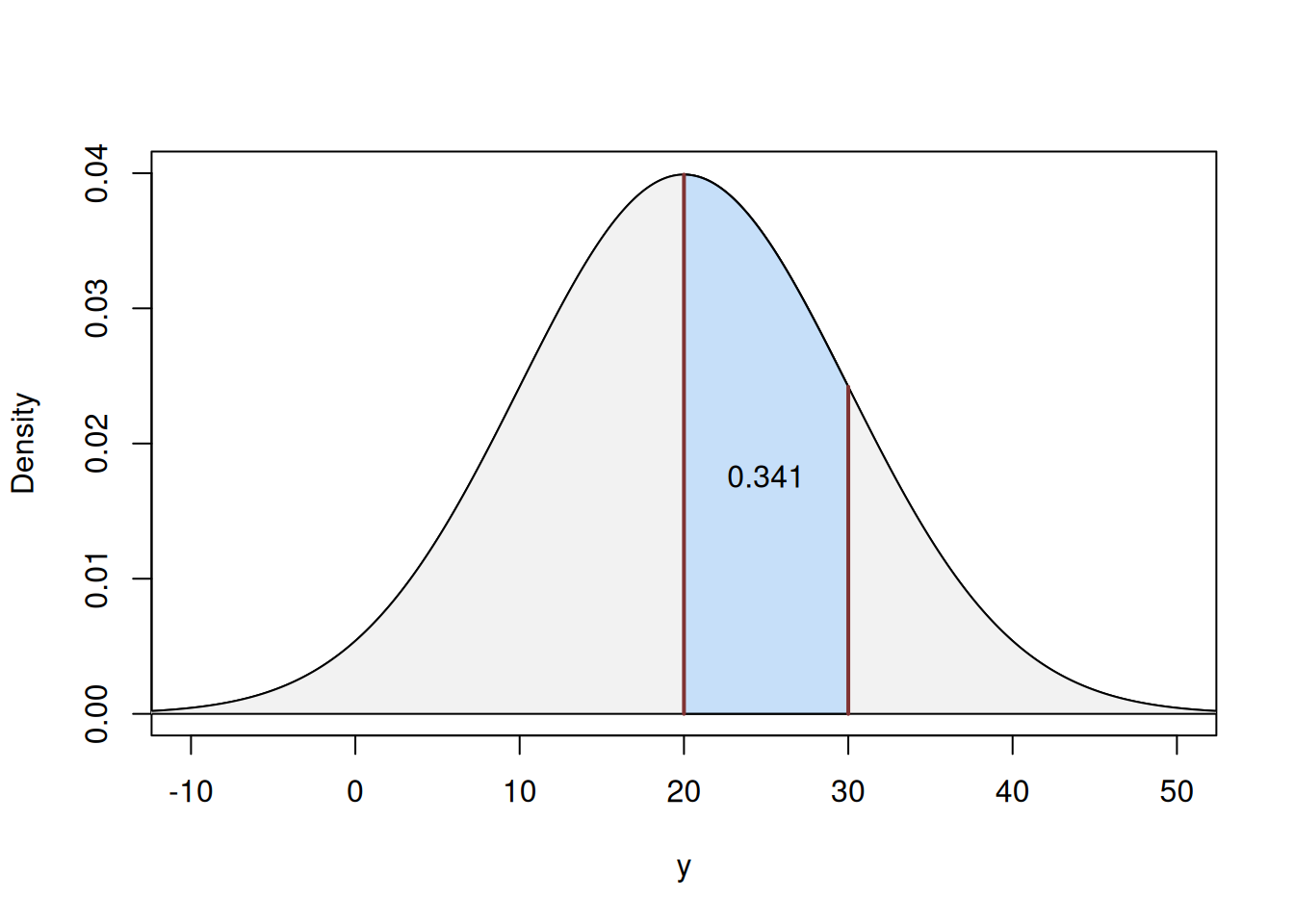
Figure 4.12: Values of PDF for the example with Normal distribution
The relation between the area in Figure 4.12 and the difference between the two points in Figure 4.11 comes directly from the definition of CDF, the latter being the function of cumulative values of the density function.
Many distributions converge to the Normal one or can be approximated by it under some circumstances. For example, as shown earlier, Binomial distribution can be approximated by the normal in some cases. More specifically, the approximation works when \(n>20\), \(n p \geq 5\) and \(n(1-p) \geq 5\). Figure 4.13 demonstrates how the normal curve (the solid red line) approximates the barplots of the Binomial distribution.
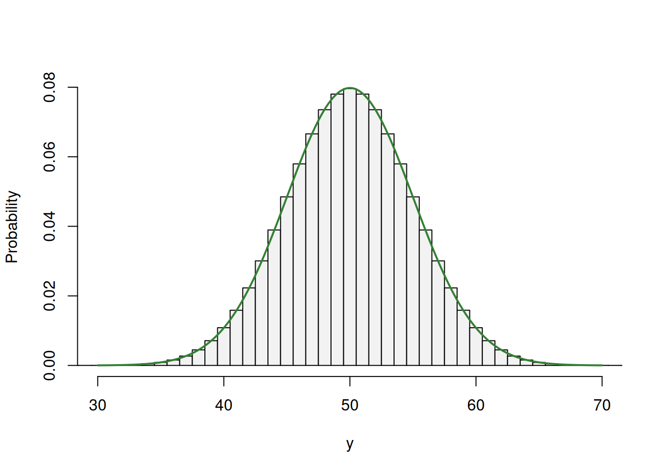
Figure 4.13: Binomial distribution and its approximation via the Normal one.
As we can see from Figure 4.13, the normal curve fits the bars of the Binomial distribution very well, which means that we can use it, for example, to compute the probability that the variable \(y\) will be equal to 41, via the formula: \[\begin{equation} \mathrm{P}(y=41) \approx \Phi(41.5, 50, 25) - \Phi(40.5, 50, 25) \tag{4.8} \end{equation}\] In the equation (4.8) by adding and subtraction 0.5, we calculate the surface of the area under the normal curve, corresponding roughly to the area of the respective bin in the barplot. We can see that this method of calculation gives a result very close to the one from the Binomial distribution:
##   Binomial     Normal
## 0.01586907 0.01584890
This calculation based on the approximation is shown visually in Figure 4.13, where the second figure is the zoomed-in area in the first one. As we can see, the area under the curve of the Normal distribution is roughly equal to the area of the bar of the Binomial distribution.
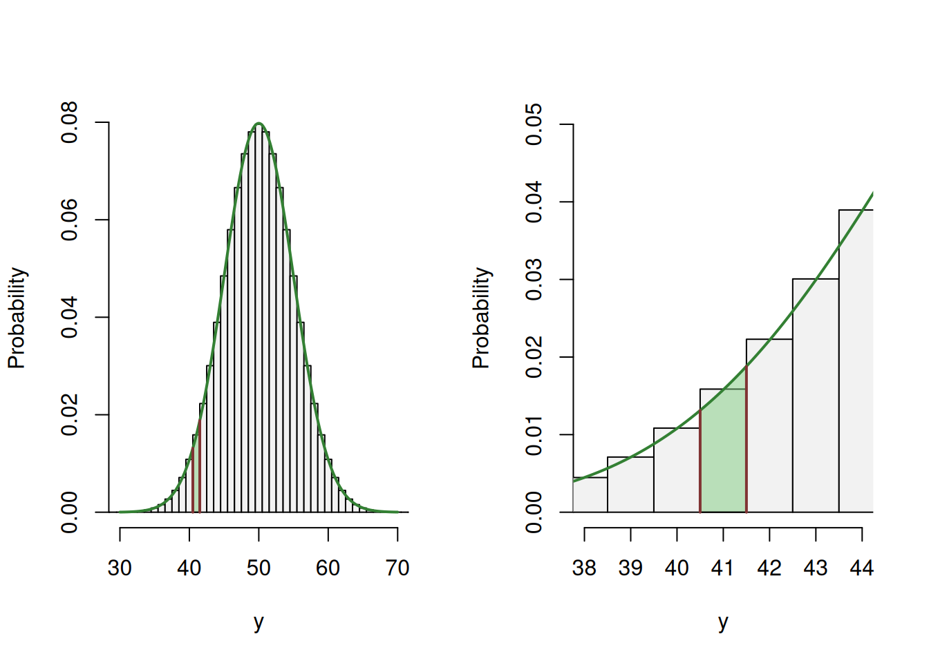
Figure 4.14: Calculating the probability based on Normal approximation.
Normal distribution is implemented in dnorm(), qnorm(), pnorm() and rnorm() functions from stats package in R.
Finally, as mentioned earlier, Normal distribution is popular among statisticians to use for the error term in a model of a type: \[\begin{equation} y_j = \mu_j + \epsilon_j, \tag{4.9} \end{equation}\] where \(\mu_j\) is some structure and \(\epsilon_j \sim \mathcal{N}(0, \sigma^2)\). The main reason for this is the ease of use of the distribution, and because it is described using its mean and variance. For example, based on (4.9), we can say that \(y_j \sim \mathcal{N}(\mu_j, \sigma^2)\), because as we remember from Chapter 2, \(\mathrm{E}(y_j)=\mathrm{E}(\mu_j) + \mathrm{E}(\epsilon_j)=\mathrm{E}(\mu_j)\). In reality, the error term of a model might not follow normal distribution, it can be more complicated and sometimes might not follow any theoretical distribution.