12.4 Hypothesis testing
In the regression context, an analyst is often interested in understanding whether a specific effect exists or not. This is usually done using the hypothesis testing instrument, which we will discuss in this section. But before we do that, we will approach this problem from a slightly non-conventional perspective, using the connection between hypothesis testing and confidence interval.
What does “effect exists” mean in statistical terms? It means that we found some evidence based on our data and model that the value of a parameter is significantly different from zero on some pre-selected level. Formally, this hypothesis is formulated as: \[\begin{equation} \begin{aligned} \mathrm{H}_0: \beta_i = 0 \\ \mathrm{H}_1: \beta_i \neq 0 \end{aligned} . \tag{12.20} \end{equation}\] where \(\beta_i\) is the true parameter in the population. The idea is to make some conclusions about what happens in population based on a specific sample of data and the estimated model.
Coming back to the example in Section 12.2, the whole hypothesis testing process implies that the distribution of the estimates of parameter for materials lies either consistently above zero or consistently below it (in our case, it is above). Figure 12.9 demonstrates the distribution we obtained from the bootstrap in the beginning of this chapter and the 95% confidence interval based on the normal approximation of the distribution.
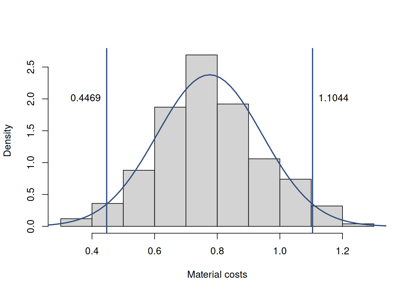
Figure 12.9: Parameter uncertainty in the estimated model for the materials variable.
The 95% confidence level corresponds to the 5% significance level. We see from Figure 12.9 that the variability of the estimate of the parameter is substantially above zero. This probably means that if we increase the sample size and continue constructing the interval, the true value will be somewhere inside and it must be not equal to zero. We use the word “probably” here because we could always make a mistake based on a specific sample or because the model was incorrectly specified. Still, we would be inclined to conclude on the 5% significance level that the effect is indeed non-zero.
Remark. In hypothesis testing, if we formulate the alternative one as inequality (as it was done in (12.20)), we cannot say whether the effect is positive or negative. We can only conclude whether it is or it is not zero on the pre-specified significance level.
If we bring this idea further, we can also conclude that the effect is not equal to 0.4 (that value is outside of the interval and in the left tail of the distribution), and surely not 1.5 (it is in the right tail). We can say that by directly looking at the confidence interval, and, arguably, it provides more information than a critical value or a p-value (we will discuss them later in this section), which would only compare the sample value with zero. But this also shows us what the hypothesis testing is all about: checking whether the tested value is inside the non-rejection interval or not. But can we make solid conclusions about the effect based on the results of the hypothesis testing?
Figure 12.10 shows the distribution of estimates of some hypothetical parameter in a regression model together with the 95% confidence interval.
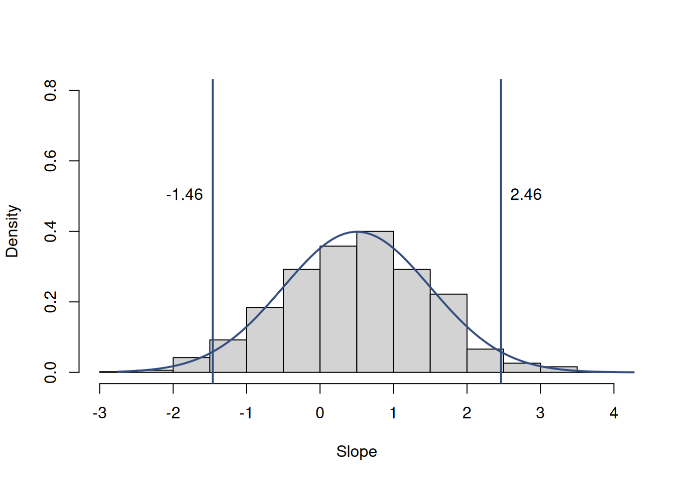
Figure 12.10: Parameter uncertainty of a hypothetical parameter.
According to Figure 12.10, the zero is included in the interval, so we would fail to reject the hypothesis that the effect is zero on the 5% significance level. This is because there is a chance that this distribution would shift to the left with the increase of the sample size and would become centered around zero. Does this mean that there is no effect? No, because we do not know what happens in population, we are making conclusions based on the limited sample and a specific model.
We can also notice that if we were to formulate a different hypothesis, for example, that the parameter is equal to one, we would fail to reject it on the 5% significance level as well. In fact, we would fail to reject the hypotheses on the 5% significance level that the true parameter equals to 0.5, 1.5 and anything between -1.46 and 2.46. Neither of this tells us anything definite about the true value of parameter. The true conclusion of hypothesis testing in this example is that we do not know what the true value of the effect is.
We personally think that the confidence interval shows this idea more clearly, than the conventional hypothesis testing, not hiding anything.
Now we will discuss the classical hypothesis testing in regression.
12.4.1 Regression parameters
The logic of hypothesis testing in regression is very similar to the one discussed in Section 7. To make it more practical, consider the regression that we have already estimated in this chapter and the coefficient for the variable materials, which equals to 0.8706. To test the hypothesis about a parameter in regression, we need to follow the procedure, described in Section 7.
First step is to formulate the null and alternative hypotheses. As discussed earlier in this section, the conventional way of doing that is by checking whether the true value of parameter is zero in the population: \[\begin{equation*} \begin{aligned} \mathrm{H}_0: \beta_i = 0 \\ \mathrm{H}_1: \beta_i \neq 0 \end{aligned} . \end{equation*}\]
Visually, the null and alternative hypotheses can be represented as shown in Figure 12.11.
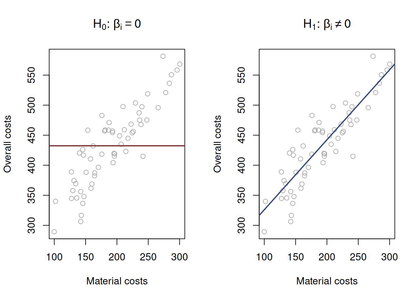
Figure 12.11: Graphical presentation of null and alternative hypothesis in regression context.
The image on the left in Figure 12.11 demonstrates how the true model could look if the null hypothesis was true - it would be just a straight line, parallel to x-axis. This would imply that with the increase of the material costs, the overall costs do not change. The image on the right in Figure 12.11 demonstrates the alternative situation, when the parameter is not equal to zero. We do not know the true model, and hypothesis testing does not tell us whether the hypothesis is true or false, but if we have enough evidence to reject H\(_0\), then we might conclude that we see an effect of one variable on the other one in the data.
After formulating the hypothesis, we select the significance level. Fro this exercise, we will choose 5%.
Then, we need to select the test to use. As discussed earlier in this chapter, if we can assume that the Central Limit Theorem holds (typically, for the linear regression estimated using the OLS, on samples of more than 50 observations, it does), we can use the Normal distribution. But given that the standard deviations of parameters are not known, and are estimated, we need to use Student’s t distribution. The formula for calculating the t-statistics is fundamentally similar to the one in Section 7.1: \[\begin{equation} t = \frac{|b_i - 0|}{s_{b_i}} , \tag{12.21} \end{equation}\] where \(b_i\) is the estimate of the parameter \(\beta_i\) and \(s_{b_i}\) is the standard error of the parameter obtained from the covariance matrix from Section 12.1. The standard deviation of the parameter is:
## [1] 0.3111558Inserting the values in formula (12.21) gives us the t-statistics value for our example: \[\begin{equation*} t = \frac{|0.871 - 0|}{0.311} \approx 2.797 \end{equation*}\] Now we need to get the critical value of the t-statistics for the selected significance value and \(n-k\) degrees of freedom, which in our case are equal to 61-5=56. We chose the significance value of 5%, and we conduct a two-sided test, so we need to split it into two parts (this would be similar to constructing a confidence interval), so we should look at the value of statistics for the 2.5% level. In R, we can get it by running:
## [1] -2.003241 2.003241In this code, we consciously provide the values of the statistics for both tails to keep the connection with the interval. If the calculated value was inside this interval, we would fail to reject the hypothesis. In our case, 2.797 lies outside of these bounds, so we can reject the H\(_0\) and conclude that based on our model and the data, we have enough evidence to say that there is an effect of material costs on the overall costs of the project.
Remark. The easier way of conducting the two sided test is to compare the t-statistics with the absolute of the critical value. In our case, we would be comparing 2.797 with 2.0032, and we would also conclude that the calculated value lies in the tails of distribution and thus we can reject the H\(_0\).
An alternative way of testing the hypothesis is by calculating the p-value and comparing it with the significance level. In that case, we would reject the H\(_0\) if the p-value is lower than the level. For our example, the p-value can be calculated using the pt() function in R:
## [1] 0.003528358Given that we conduct the two-tail test, this p-value needs to be multiplied by 2 to get approximately 0.00706. The conclusion that we can draw from this is that we reject the null hypothesis on the 5% significance level.
All of this is done automatically by R if we estimate the model using the basic lm() function from the stats package:
##
## Call:
## lm(formula = overall ~ materials + size + projects + year, data = SBA_Chapter_11_Costs)
##
## Residuals:
##      Min       1Q   Median       3Q      Max
## -101.198  -30.443   -2.157   26.032  108.496
##
## Coefficients:
##              Estimate Std. Error t value Pr(>|t|)
## (Intercept)  614.3227  4337.3590   0.142  0.88788
## materials      0.8706     0.3112   2.798  0.00704 **
## size           1.3471     0.6989   1.928  0.05898 .
## projects      -1.5921     3.7971  -0.419  0.67660
## year          -0.1602     2.1621  -0.074  0.94121
## ---
## Signif. codes:  0 '***' 0.001 '**' 0.01 '*' 0.05 '.' 0.1 ' ' 1
##
## Residual standard error: 43.42 on 56 degrees of freedom
## Multiple R-squared:  0.749,  Adjusted R-squared:  0.7311
## F-statistic: 41.77 on 4 and 56 DF,  p-value: 3.415e-16
The output above shows the estimates of parameters, the standard errors, the t-values and p-values (called “Pr(>|t|)”).
Remark. When working with p-values, there is a temptation to not select the significance level before conducting the test or changing it after obtaining the results. This is one of the typical mistakes that can lead to so called p-hacking, where the interpretation of the results of the experiment are amended to fit better to preferences of analyst. This temptation should be resisted! This and other mistakes related to p-values and hypothesis testing were discussed in Subsection 7.1.1.
The context of regression also provides a great example, why we never accept the null hypothesis and why in the case of “Fail to reject H\(_0\)”, we should not remove a variable (unless we have more fundamental reasons for doing that). Consider an example, where the estimated parameter \(b_1=0.5\), and its standard error is \(s_{b_1}=1\), we estimated a simple linear regression on a sample of 30 observations, and we want to test, whether the parameter in the population is zero (hypothesis (12.20)) on 5% significance level. Inserting the values in formula (12.21), we get: \[\begin{equation*} \frac{|0.5 - 0|}{1} = 0.5, \end{equation*}\] with the critical value for two-tailed test of \(t_{0.025}(30-2)\approx 2.05\). Comparing t-value with the critical one, we would conclude that we fail to reject H\(_0\) and thus the parameter is not statistically different from zero. There is a temptation to remove it from the model, but this would be fundamentally wrong. And here is why.
Consider testing another hypothesis for the same parameter: \[\begin{equation*} \begin{aligned} \mathrm{H}_0: \beta_1 = 1 \\ \mathrm{H}_1: \beta_1 \neq 1 \end{aligned} . \end{equation*}\] The procedure is the same, the calculated t-value is: \[\begin{equation*} \frac{|0.5 - 1|}{1} = 0.5, \end{equation*}\] which leads to exactly the same conclusion as before: on 5% significance level, we fail to reject the new H\(_0\), so the value is not distinguishable from 1. So, which of the two conclusions is correct? Is it zero or is it one?
The correct answer is “we do not know”. The non-rejection region just tells us that the uncertainty about the parameter is so high that it also includes the value of interest (0 in case of the classical regression analysis or 1 in the case of the second hypothesis). If we constructed the confidence interval for this problem, we would not have such confusion, as we would conclude that on 5% significance level the true parameter lies in the region \((-1.46, 2.46)\) and can be any of the numbers between them.
12.4.2 Regression line
Finally, in regression context, we can test another hypothesis, which becomes useful, when many parameters of the model are very close to zero and seem to be insignificant on the selected level: \[\begin{equation} \begin{aligned} \mathrm{H}_0: \beta_1 = \beta_2 = \dots = \beta_{k-1} = 0 \\ \mathrm{H}_1: \beta_1 \neq 0 \vee \beta_2 \neq 0 \vee \dots \vee \beta_{k-1} \neq 0 \end{aligned} , \tag{12.22} \end{equation}\] which translates into normal language as: \[\begin{equation*} \begin{aligned} \mathrm{H}_0: \text{ all parameters (except for intercept) are equal to zero}\\ \mathrm{H}_1: \text{ at least one parameter is not equal to zero} \end{aligned} . \end{equation*}\] This hypothesis is only needed when you have a model with many statistically insignificant variables and want to see if overall the model explains anything. This is done using F-test, which can be calculated based on sums of squares (discussed in Subsection 10.4.1): \[\begin{equation*} F = \frac{ SSR / (k-1)}{SSE / (n-k)} \sim F(k-1, n-k) , \end{equation*}\] where the sums of squares are divided by their degrees of freedom. The test is conducted in the similar manner as any other test (see Section 7): after choosing the significance level, we calculate the F-value and then either select the critical value of F for the specific degrees of freedom, or compare the significance level with the p-value from the test to make a conclusion about the null hypothesis.
There are several things to consider about the F-test in regression:
- It is not very useful, when at least one parameter is statistically significant. It only becomes useful in difficult situations of poor fit.
- The test on its own does not tell if the model is good or bad, adequate or not, etc.
- And the F value and related p-value are not comparable with respective values of another models.
Visually, this test checks, whether in the true model the slope of the line on the plot of actuals vs fitted is different from zero. An example with the same costs model is provided in Figure 12.12.
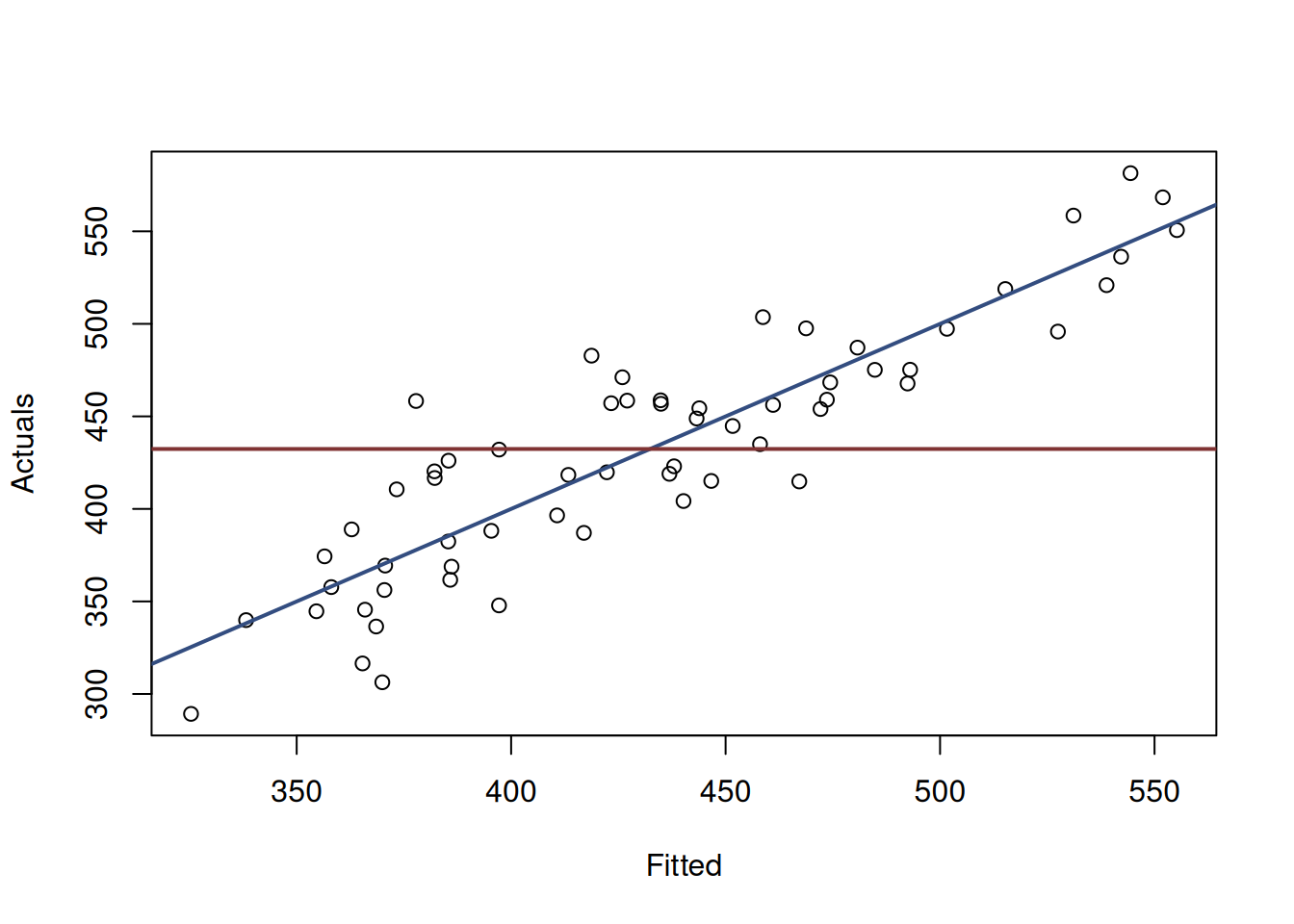
Figure 12.12: Graphical presentation of F-test for regression model.
What the F-test is about, is whether in the true model (population data) the blue line coincides with the red line (i.e. the slope is equal to zero, which is only possible, when all parameters are zero). If given the data and the model, we have enough evidence to reject the null hypothesis, then this means that the slopes are probably different on the selected significance level.
Here is an example with the costs model discussed in this chapter with the pre-selected significance level of 5%:
# Estimate the regression using lm
costsModelMLRLm <- lm(overall~materials+size+projects+year,
                      data=SBA_Chapter_11_Costs)
# Get summary statistics
costsModelMLRF <- summary(costsModelMLRLm)$fstatistic
# Extract the F-value
costsModelMLRF[1]
## value
## 41.77388## [1] 2.536579In the output above, the critical value is lower than the calculated, so we can reject the H\(_0\), which means that there is something in the model that explains the variability of the overall costs. Alternatively, we could focus on the p-value:
# p-value from the test
pf(costsModelMLRF[1], costsModelMLRF[2], costsModelMLRF[3], lower.tail=FALSE)
## value
## 3.414938e-16We see that the the p-value is lower than the significance level of 5%, so we reject the H\(_0\) on that level and come to the same conclusion as above. All of this is also provided by default in the summary of the model estimated using the lm() function:
##
## Call:
## lm(formula = overall ~ materials + size + projects + year, data = SBA_Chapter_11_Costs)
##
## Residuals:
##      Min       1Q   Median       3Q      Max
## -101.198  -30.443   -2.157   26.032  108.496
##
## Coefficients:
##              Estimate Std. Error t value Pr(>|t|)
## (Intercept)  614.3227  4337.3590   0.142  0.88788
## materials      0.8706     0.3112   2.798  0.00704 **
## size           1.3471     0.6989   1.928  0.05898 .
## projects      -1.5921     3.7971  -0.419  0.67660
## year          -0.1602     2.1621  -0.074  0.94121
## ---
## Signif. codes:  0 '***' 0.001 '**' 0.01 '*' 0.05 '.' 0.1 ' ' 1
##
## Residual standard error: 43.42 on 56 degrees of freedom
## Multiple R-squared:  0.749,  Adjusted R-squared:  0.7311
## F-statistic: 41.77 on 4 and 56 DF,  p-value: 3.415e-16
The summary for the alm() does not provide this information because it has a different philosophy behind it (likelihood, which we will discuss in Chapter 16).