3.5 Poisson distribution (Modelling arrivals)
Consider a situation, when we want to model an arrival of patients in a hospital for each hour of day. In that case, they arrive for different reasons: some have fractures, others have headaches, some come because they sneezed and the others are there because they are seriously ill. There is potentially a lot of people that could come to the hospital (the whole population living in the area), but typically only few of them will show up in each specific hour. Furthermore, all these people are typically not related (unless there was an event that caused a specific condition to a group of people, such as a big pub fight) and arrive at random. In this example, we could argue that the process of arrival is memoryless, because the arrivals of different patients are not related. For the probability theory, this implies that the probability that a patient arrives in a specific period of time should be independent of when the previous patient arrived. Mathematically, this is represented as: \[\begin{equation} \mathrm{P}(t > \tau_1 + \tau_2) = \mathrm{P}(t > \tau_1)\mathrm{P}(t > \tau_2), \tag{3.10} \end{equation}\] where \(t\) is the waiting time until the next arrival, and \(\tau_1\) and \(\tau_2\) are waiting times. The formula (3.10) shows that the probability that we will wait more than \(\tau_1\) and \(\tau_2\) is just equal to the product of probabilities of waiting for more than \(\tau_1\) and more than \(\tau_2\). The formula relies on the independence of probabilities (discussed in Chapter 2). From the mathematical point of view, there is a function that supports the property (3.10) - it is exponent: \[\begin{equation} e^{\tau_1 + \tau_2} = e^{\tau_1} e^{\tau_2} . \tag{3.11} \end{equation}\] Based on this principle of memorylessness (and based on the Exponential distribution, which we will discuss in Section 4.5), Poisson distribution is derived. It is a discrete distribution, which is used for modelling number of patients arriving at specific time intervals, based on the average number of arrivals \(\lambda\). Its PMF has the shape shown in Figure 3.8.
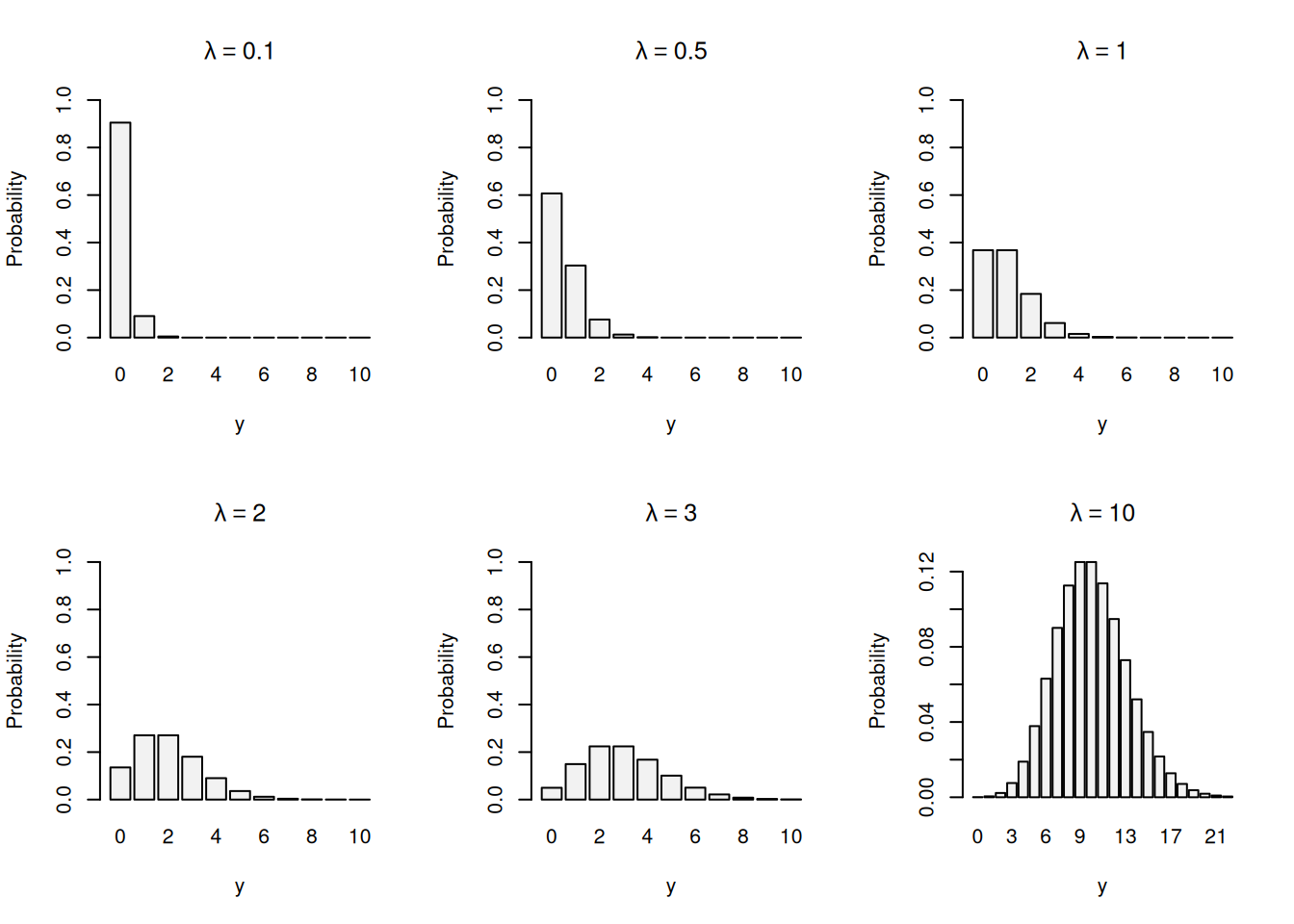
Figure 3.8: Probability Mass Function of Poisson distribution with different values of \(\lambda\).
From the graphs in Figure 3.8, we can make several observations:
- Zeroes are natural in Poisson distribution. This means that there is a chance that nobody will come in the next hour.
- With the increase of the average number of arrivals \(\lambda\), the chance to have more patients arriving increases. For example, with \(\lambda=0.1\), the probability of having no patients is approximately 0.9, while in case of \(\lambda=1\), it is approximately 0.4.
- With the increase of \(\lambda\), the shape of distribution becomes closer to the Normal one (discuss in Section 4.3).
Mathematically, the PMF of Poisson distribution is represented as: \[\begin{equation} f(y, \lambda) = \frac{\lambda^y e^{-\lambda}}{y!} , \tag{3.12} \end{equation}\] where \(e\) is the Euler’s constant. The part \(e^{-\lambda}\) represents the memoryless arrivals of patients. The Poisson distribution is characterised as \(\mathcal{Pois}(\lambda)\) and has an additional property that its expectation is equal to variance: \[\begin{equation} \mathrm{E}(y) = \mathrm{V}(y) = \lambda , \tag{3.13} \end{equation}\] which makes it convenient to work with and easy to estimate. If we have the parameters of the Poisson distribution, we can calculate probabilities for a variety of situations or generate quantiles - depending on what we need specifically. For example, for scheduling purposes we might need to understand what is the probability of having more than zero but up to four patients in any specific hour. Assume that based on the available data we estimated that \(\hat{\lambda}=2\). In this situation we need to either use PMF or the CDF to calculate the following probability: \[\begin{equation} \begin{aligned} \mathrm{P}(0 < y \leq 4) = & \mathrm{P}(y=1) + \mathrm{P}(y=2) + \mathrm{P}(y=3) + \mathrm{P}(y=4) = \\ & \mathrm{P}(y \leq 4) - \mathrm{P}(y=0) \end{aligned} . \tag{3.14} \end{equation}\]
The first line in (3.14) shows how the probability can be calculated via the PMF, while the second one is for the CDF. They both can be calculated in R via:
## [1] 0.8120117## [1] 0.8120117where dpois() is the PMF and ppois() is the CDF of the Poisson distribution. Mathematically, the CDF of the Poisson distributions is written as:
\[\begin{equation}
F(y, \lambda) = e^{-\lambda} \sum_{j=0}^{y} \frac{\lambda^j }{j!} ,
\tag{3.15}
\end{equation}\]
for integer values of \(y\). Finally, we could get quantiles of the distribution for the specified probability. In R, this is done via the qpois() function. For example, here is the 0.95 quantile for the Poisson distribution with \(\hat{\lambda}=2\):
## [1] 5Remark. When identifying a suitable distribution, Poisson has several distinct characteristics:
- There are many trials (in our example with the hospital, many people live in the area).
- There is a small chance that each specific patient will arrive in a specific hour (number of patients arriving at the hospital each hour is small in comparison with the population).
- Each specific event is independent of the others (memorylessness property: a patient arrives independent of another one).
These three criteria can be used to identify Poisson distribution in practice.