17.1 Bias-variance tradeoff
17.1.1 Graphical explanation
In order to better understand, why we need to bother with model selection, combinations and advanced estimators, we need to understand the principle of bias-variance tradeoff. Consider a simple example of relation between fuel consumption of a car and the engine size based on the mtcars dataset in R (Figure 17.1):
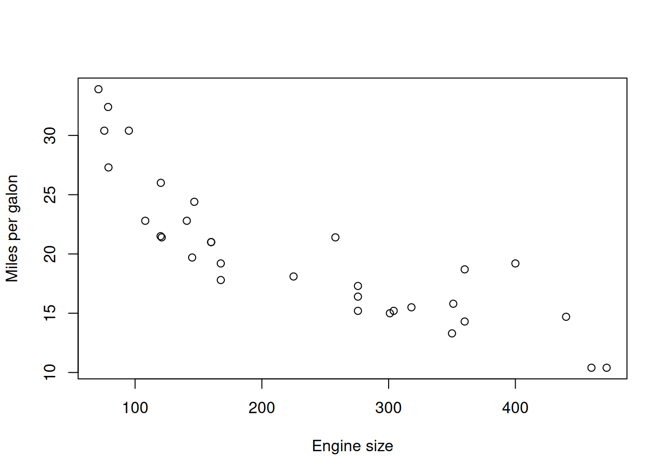
Figure 17.1: Fuel consumption vs engine size
The plot in Figure 17.1 demonstrates clear non-linearity. Indeed, we would expect the relation between these variables to be non-linear in real life: it is difficult to imagine the situation, where a car with no engine will be able to drive at all. On the other hand, a car with a huge engine will still be able to drive some distance, although probably very small. The linear model would assume that the “no engine” case would correspond to the value of approximately 30 miles per gallon (the intersection with y-axis), while the case of “huge engine” would probably result in negative mileage. So, the theoretically suitable model should be multiplicative, which for example can be formulated in logarithms: \[\begin{equation} \log mpg_j = \beta_0 + \beta_1 \log disp_j + \epsilon_j , \tag{17.1} \end{equation}\] where \(mpg_j\) is the miles per galon of a car and \(disp_j\) is the displacement (size) of engine. We will assume for now that this is the “true model”, which would fit the data in the following way if we knew all the data in the universe (Figure 17.2):
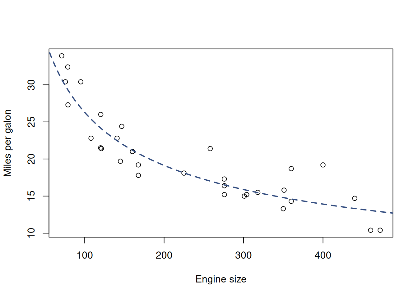
Figure 17.2: Fuel consumption vs engine size and the true model
While being wrong, we could still use the linear model to capture some relations in some parts of the data. It would not be a perfect fit (and would have some issues in the tails of our data), but it would be an acceptable approximation of the true model in some situations. If we vary the sample, we will see how the model would behave, which would help us in understanding of the uncertainty associated with it (Figure 17.3).
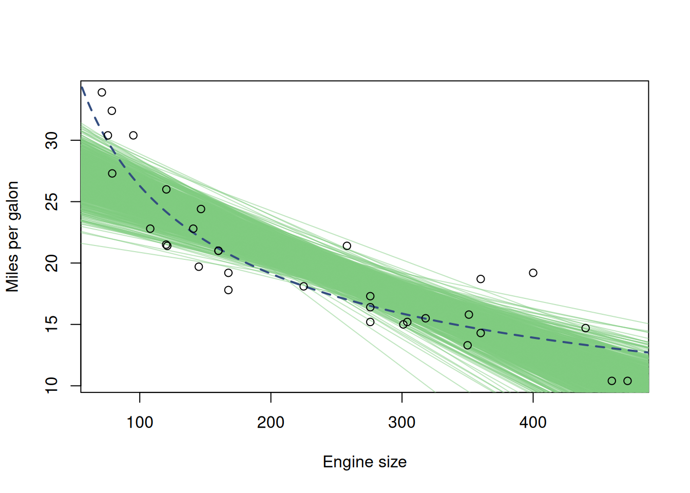
Figure 17.3: Fuel consumption vs engine size, the true and the linear models
Figure 17.3 demonstrates the situation, where the linear model was fit to randomly peaked sub-samples of the original data. We can see that the linear model would exhibit some sort of bias in comparison with the true one: it is consistently above the true model in the region in the middle and is consistently below it in the tails of the sample.
Alternatively, we could fit a high order polynomial model to approximate the data and repeat the same procedure with sub-samples as before (Figure 17.4):
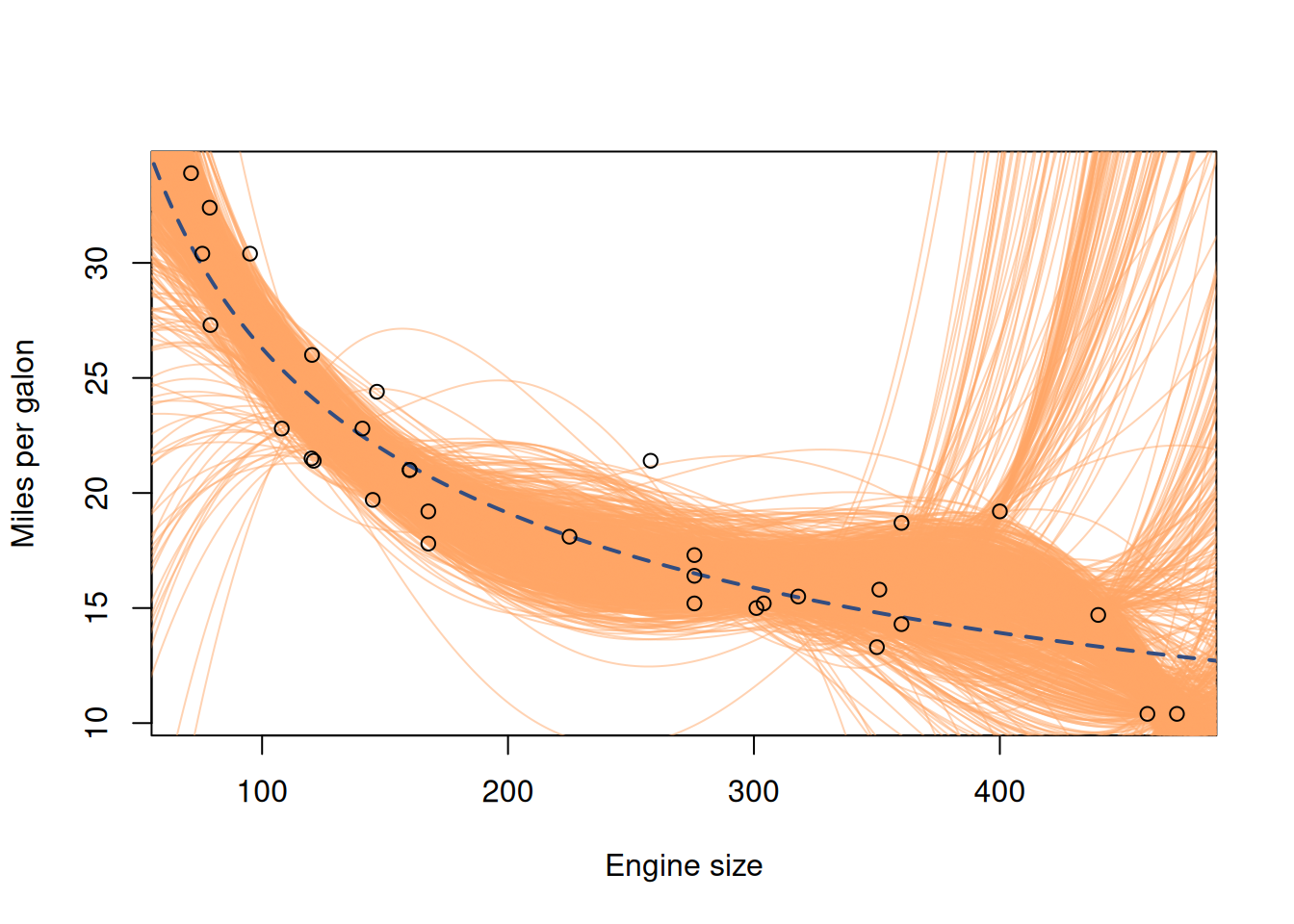
Figure 17.4: Fuel consumption vs engine size, the true, the linear and the polynomial models.
The new polynomial model on the plot in Figure 17.4 has a lower bias than the linear one, because on average it is closer to the true model in sample, getting closer to the green line (true model) even in the tails. However, it is also apparent that it has higher variability. This is because it is a more complex model than the linear one: it includes more variables (polynomial terms), making it more sensitive to specific observations in the sample. If we were to introduce even more polynomial terms, the model would have even more variance around the true model than before (Figure 17.5).
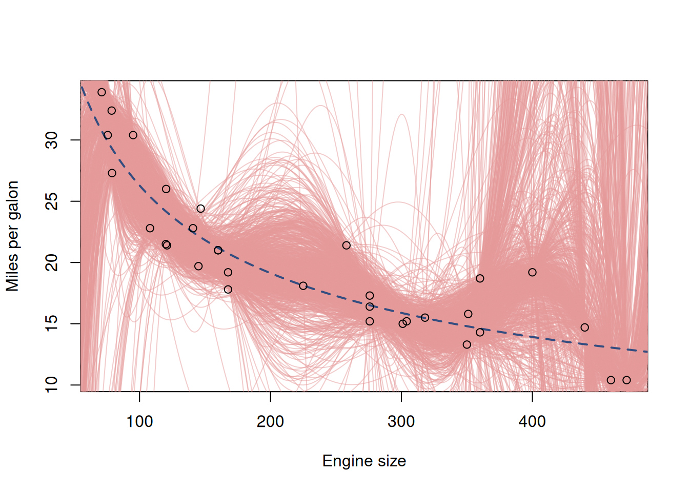
Figure 17.5: Fuel consumption vs engine size, the true and the polynomial (7th order) models
The model on plot in Figure 17.5 exhibits even higher variance in comparison with the true model, but it is still less biased than the linear model. The pattern that we observe in this demonstration is that the variance of the model in comparison with the true one increases with the increase of complexity, while the bias either decreases or does not change substantially. This is bias-variance tradeoff in action. It is the principle that states that with the increase of complexity of model, its variance (with respect to the true one) increases, while the bias decreases. This implies that typically you cannot minimise both variance and bias at the same time - depending on how you formulate and estimate a model, it will either have bigger variance or a bigger bias. This principle can be applied not only to models, but also to estimates of parameters or to forecasts from the models. It is one of the fundamental basic modelling principles.
17.1.2 Mathematical explanation
Mathematically, it is represented for an estimate as parts of Mean Squared Error (MSE) of that estimate (we drop the index of observations \(j\) in \(\hat{y}_j\) for convenience): \[\begin{equation} \mathrm{MSE} = \mathrm{Bias}(\hat{y})^2 + \mathrm{V}(\hat{y}) + \sigma^2 , \tag{17.2} \end{equation}\] where \(\hat{y}\) is the fitted value of our model, \(\mathrm{Bias}(\hat{y})=\mathrm{E}(\mu_y-\hat{y})\), \(\mathrm{V}(\hat{y})=\mathrm{E}\left((\mu_y-\hat{y})^2\right)\), \(\mu_y\) is the fitted value of the true model, and \(\sigma^2\) is the variance of the white noise of the true model.
Proof. The Mean Squared Error of a model by definition is the expectation of the squared difference between the actual and the fitted values: \[\begin{equation} \mathrm{MSE} = \mathrm{E}\left((y -\hat{y})^2\right) = \mathrm{E}\left((\mu_y +\epsilon -\hat{y})^2\right) \tag{17.3} \end{equation}\] The expectation of square of sum above can be expanded as: \[\begin{equation} \begin{aligned} \mathrm{MSE} = & \mathrm{E}\left(\left(\mu_y +\epsilon -\hat{y} +\mathrm{E}(\hat{y}) -\mathrm{E}(\hat{y})\right)^2\right) =\\ & \mathrm{E}\left((\mu_y -\mathrm{E}(\hat{y}))^2\right) +\\ & \mathrm{E}\left((\mathrm{E}(\hat{y}) -\hat{y})^2\right) +\\ & \mathrm{E}(\epsilon^2) +\\ & 2\mathrm{E}\left((\mu_y -\mathrm{E}(\hat{y})) \epsilon \right) +\\ & 2\mathrm{E}\left((\mathrm{E}(\hat{y}) -\hat{y}) \epsilon \right) +\\ & 2\mathrm{E}\left((\mu_y -\mathrm{E}(\hat{y}))(\mathrm{E}(\hat{y}) -\hat{y}) \right) \end{aligned} \tag{17.4} \end{equation}\] We now can consider each element of the sum of squares in (17.4) to understand what they are equal to. We start with the first one, which can be expanded to: \[\begin{equation} \mathrm{E}\left((\mu_y -\mathrm{E}(\hat{y}))^2\right) = \mathrm{E}(\mu_y^2) -2 \mathrm{E}(\mu_y \mathrm{E}(\hat{y})) + \mathrm{E}(\mathrm{E}(\hat{y})^2). \tag{17.5} \end{equation}\] Given that \(\mu_y\) is the value of the model in the population, which is fixed, its expectation will be equal to itself. In addition, the expectation of expectation is just an expectation: \(\mathrm{E}(\mathrm{E}(\hat{y})^2)=\mathrm{E}(\hat{y})^2\). This leads to the following, which is just the bias of the estimated model: \[\begin{equation} \begin{aligned} \mathrm{E}\left((\mu_y -\mathrm{E}(\hat{y}))^2\right) = & \mu_y^2 -2 \mu_y \mathrm{E}(\hat{y}) + \mathrm{E}(\hat{y})^2 = \\ & (\mu_y -\mathrm{E}(\hat{y}))^2 = \mathrm{Bias}(\hat{y})^2 \end{aligned} \tag{17.6} \end{equation}\] The second term in (17.4) is the variance of the model (by the definition of variance): \[\begin{equation} \mathrm{E}\left((\mathrm{E}(\hat{y}) -\hat{y})^2\right) = \mathrm{V}(\hat{y}) \tag{17.7} \end{equation}\] The third term is equal to the variance of the error term as long as the expectation of the error is zero (which is one of the conventional assumptions, discussed in Subsection 15.2.3): \[\begin{equation} \mathrm{E}(\epsilon^2) = \sigma^2 \tag{17.8} \end{equation}\] The more complicated thing is to show that the the other three elements are equal to zero. For the elements number four and five, we can use the assumption that the error term of the true model is independent of anything else (see discussion in Section 15.2), leading respectively to: \[\begin{equation} \mathrm{E}\left((\mu_y -\mathrm{E}(\hat{y})) \epsilon \right) = \mathrm{E}(\mu_y -\mathrm{E}(\hat{y})) \times \mathrm{E}(\epsilon) \tag{17.9} \end{equation}\] and \[\begin{equation} \mathrm{E}\left((\mathrm{E}(\hat{y}) -\hat{y}) \epsilon \right) = \mathrm{E}(\mathrm{E}(\hat{y})-\hat{y}) \times \mathrm{E}(\epsilon) . \tag{17.10} \end{equation}\] Given that \(\mathrm{E}(\epsilon)=0\) due to one of the assumptions (Subsection 15.2.3), both terms will be equal to zero. Finally, the last term can be expanded to: \[\begin{equation} \begin{aligned} \mathrm{E}\left((\mu_y -\mathrm{E}(\hat{y}))(\mathrm{E}(\hat{y}) -\hat{y}) \right) = & \mathrm{E}(\mu_y \mathrm{E}(\hat{y}) -\mu_y \hat{y} -\mathrm{E}(\hat{y})\mathrm{E}(\hat{y}) +\mathrm{E}(\hat{y})\hat{y}) = \\ & \mu_y \mathrm{E}(\hat{y}) -\mu_y \mathrm{E}(\hat{y}) -\mathrm{E}(\hat{y})^2 +\mathrm{E}(\hat{y})^2 = \\ & 0 \end{aligned} \tag{17.11} \end{equation}\] So, this means that the last three terms in (17.4) are equal to zero and thus, inserting (17.5), (17.6) and (17.7) in (17.4), we get: \[\begin{equation*} \mathrm{MSE} = \mathrm{Bias}(\hat{y})^2 + \mathrm{V}(\hat{y}) + \sigma^2 \end{equation*}\]
The similar mathematical formula holds for any other estimate, for example for an estimate of parameter. What this formula tells us is that there are two forces in the MSE of estimate that impact its value. Minimisation MSE does not imply that we reduce both of them, but most probably we are reducing one at the cost of another. The classical plot based on this looks as shown in Figure 17.6.
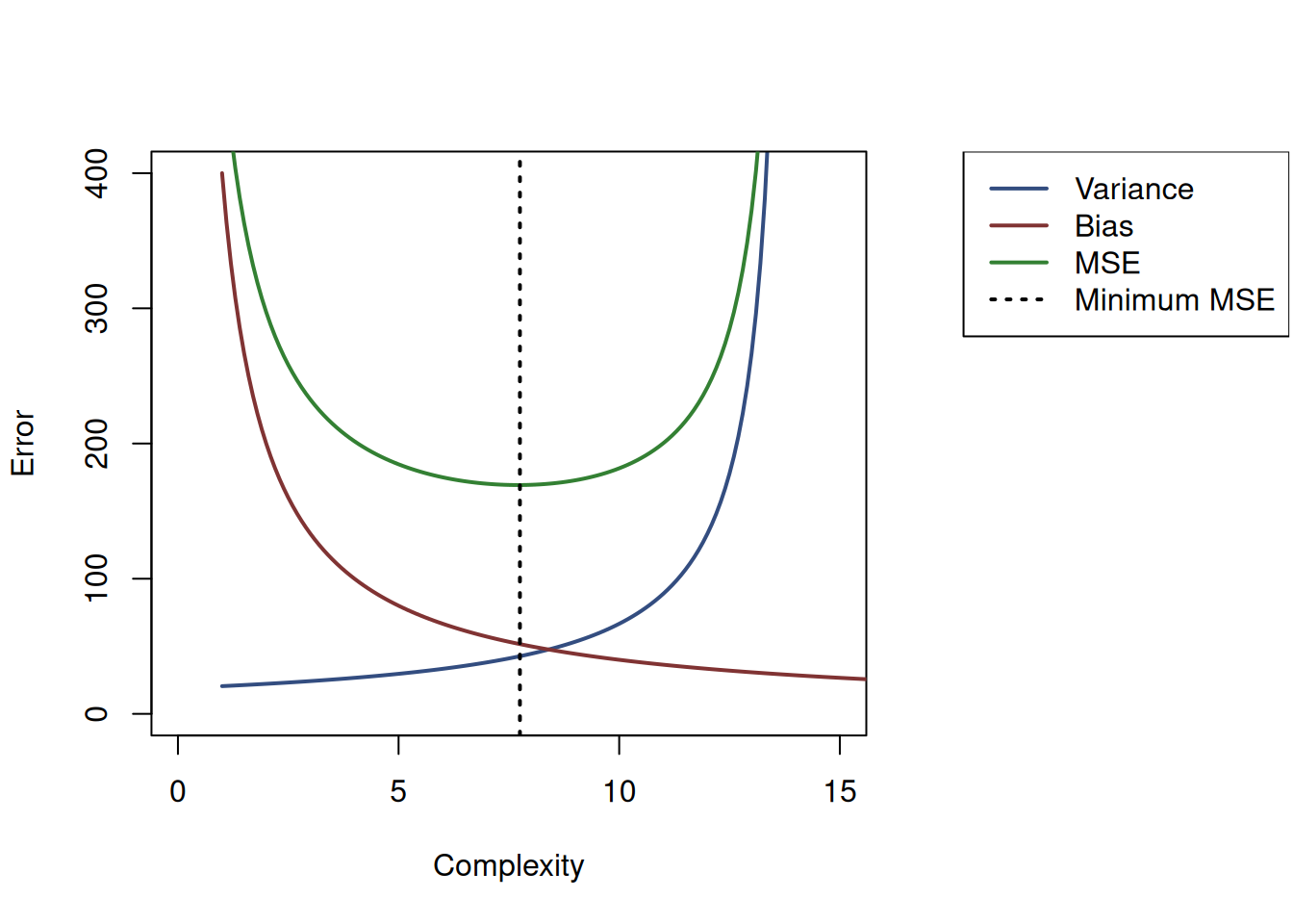
Figure 17.6: Bias, Variance and MSE as functions of model complexity.
This plot shows the basic principles: with increase of complexity, the bias of estimate decreases, but its variance increases. There is typically the specific type of model (the point on Complexity axis) that minimises MSE (the vertical line on the plot), which will have some combination of variance and bias. But in practice, this point does not guarantee that we will have an accurate adequate model. In some situations we might prefer moving to the left on the plot in Figure 17.6, sacrificing unbiasedness of model to get the reduced variance. The model selection, model combinations and regularisation methods all aim to find the sweet spot on the plot for the specific sample available to the analyst.
The bias-variance trade-off is also related to the discussion we had in Subsection 6.4.5: having a more biased but more efficient estimate of parameter (thus going to the left in Figure 17.6) might be more desirable than having the unbiased but inefficient estimate. This is because on small samples the former estimate will be typically closer to the true value than the latter one. This explains why model selection, model combinations and regularisation are important topics and have become so popular over the last few decades: they all allow deciding, where to be in the bias-variance trade-off in order to produce more accurate estimates of parameters based on the available sample of data.