14.1 Example of application
Consider, for example, the stopping distance vs speed of the car, the case we have discussed in the previous sections. This sort of relation in reality is non-linear. We know from physics that the distance travelled by car is proportional to the mass of car, the squared speed and inversely proportional to the breaking force: \[\begin{equation} distance \propto \frac{mass}{2 breaking} \times speed^2. \tag{14.1} \end{equation}\] If we use the linear function instead, then we might fail in capturing the relation correctly. Here is how the linear regression looks like, when applied to the data (Figure 14.1).
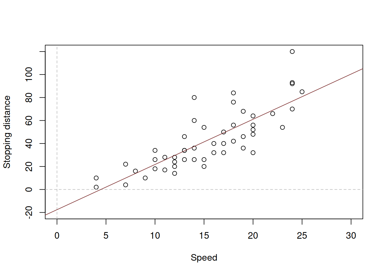
Figure 14.1: Speed vs stopping distance and a linear model
The model on the plot in Figure 14.1 is misleading, because it predicts that the stopping distance of a car, travelling with speed less than 4mph will be negative. Furthermore, the modelunderestimates the real stopping distance for cars with higher speed. If a decision is made based on this model, then it will be inevitably wrong and might potentially lead to serious repercussions in terms of road safety. Given the relation (14.1), we should consider a non-linear model. In this specific case, we should consider the model of the type: \[\begin{equation} distance = \beta_0 speed^{\beta_1} \times (1+\epsilon). \tag{14.2} \end{equation}\] The multiplication of speed by the error term is necessary, because the effect of randomness will have an increasing variability with the increase of speed: if the speed is low, then the random factors (such as road conditions, breaks condition etc) will not have a strong effect on distance, while in case of the high speed these random factors might lead either to the serious decrease or increase of distance (a car on a slippery road, stopping from 50mph will have much longer distance than the same car on a dry road). Note that I have left the parameter \(\beta_1\) in (eq:speedDistanceModel) and did not set it equal to two. This is done for the case we want to estimate the parameter based on the data. The problem with the model (14.2) is that it is difficult to estimate due to the non-linearity. In order to resolve this problem, we can linearise it by taking logarithms of both sides, which will lead to: \[\begin{equation} \log (distance) = \log \beta_0 + \beta_1 \log (speed) + \log(1+\epsilon). \tag{14.3} \end{equation}\] If we substituted every element with \(\log\) in (14.3) by other names (e.g. \(\log(\beta_0)=\beta^\prime_0\) and \(\log(speed)=x\)), it would be easier to see that this is a linear model, which can be estimated via OLS. This type of model is called “log-log”, reflecting that it has logarithms on both sides. Even the data will be much better behaved if we use logarithms in this situation (see Figure 14.2).
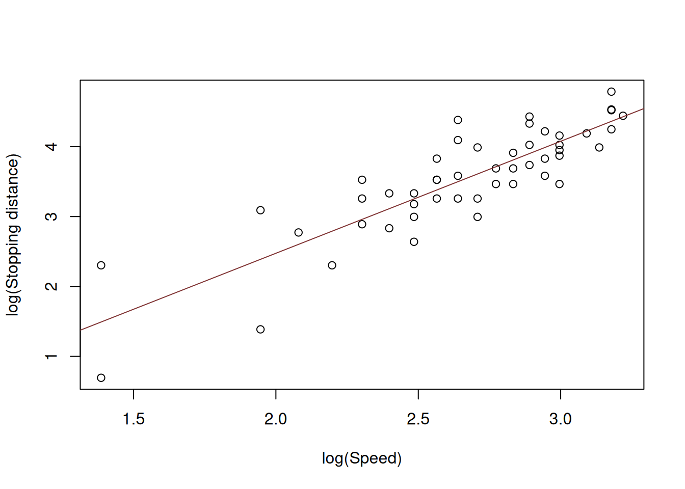
Figure 14.2: Speed vs stopping distance in logarithms
What we want to see on Figure 14.2 is the linear relation between the variables with points having fixed variance. However, in our case we can notice that the variance of the stopping distances does not seem to be stable: the variability around 2.0 is higher than the variability around 3.0. This might cause issues in the model due to violation of assumptions (see Section 15). For now, we acknowledge the issue but do not aim to fix it. And here how the model (14.3) can be estimated using R:
The values of parameters of this model will have a different meaning than the parameters of the linear model. Consider the example with the model above:
## Response variable: logdist
## Distribution used in the estimation: Normal
## Loss function used in estimation: MSE
## Coefficients:
##             Estimate Std. Error Lower 2.5% Upper 97.5%
## (Intercept)  -0.7297     0.3758    -1.4854       0.026
## log(speed)    1.6024     0.1395     1.3218       1.883 *
##
## Error standard deviation: 0.4053
## Sample size: 50
## Number of estimated parameters: 2
## Number of degrees of freedom: 48
## Information criteria:
##     AIC    AICc     BIC    BICc
## 55.5318 56.0536 61.2679 62.2884
The value of parameter for the variable log(speed) now does not represent the marginal effect of speed on distance, but rather shows the elasticity, i.e. if the speed of a car increases by 1%, the travel distance will increase on average by 1.6%.
In order to analyse the fit of the model on the original data, we would need to produce fitted values and exponentiate them. Note that in this case they would correspond to geometric rather than arithmetic means:
plot(cars, xlab="Speed", ylab="Stopping distance")
lines(cars$speed,exp(fitted(slmSpeedDistanceModel01)),col=2)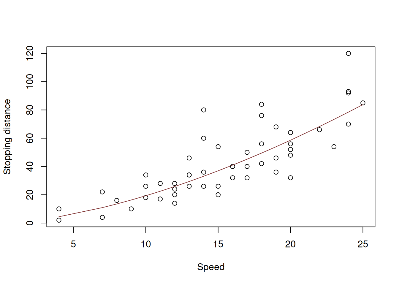
Figure 14.3: Speed vs stopping distance and the log-log model fit.
The resulting model in Figure 14.3 is the power function, which exhibits the increase in speed of change of one parameter with a linear change of another one. Note that technically speaking, the log-log model only makes sense, when the data is strictly positive. If it also contains zeroes (the speed is zero, thus the stopping distance is zero), then some other transformations might be in order. For example, we could square the speed in the model and try constructing the linear model, aligning it better with the physical model (14.1): \[\begin{equation} distance = \beta_0 + \beta_1 speed^2 + \epsilon . \tag{14.4} \end{equation}\] The issue of this model would be that the error term is additive and thus the model would assume that the variability of the error does not change with the speed, which is not realistic.
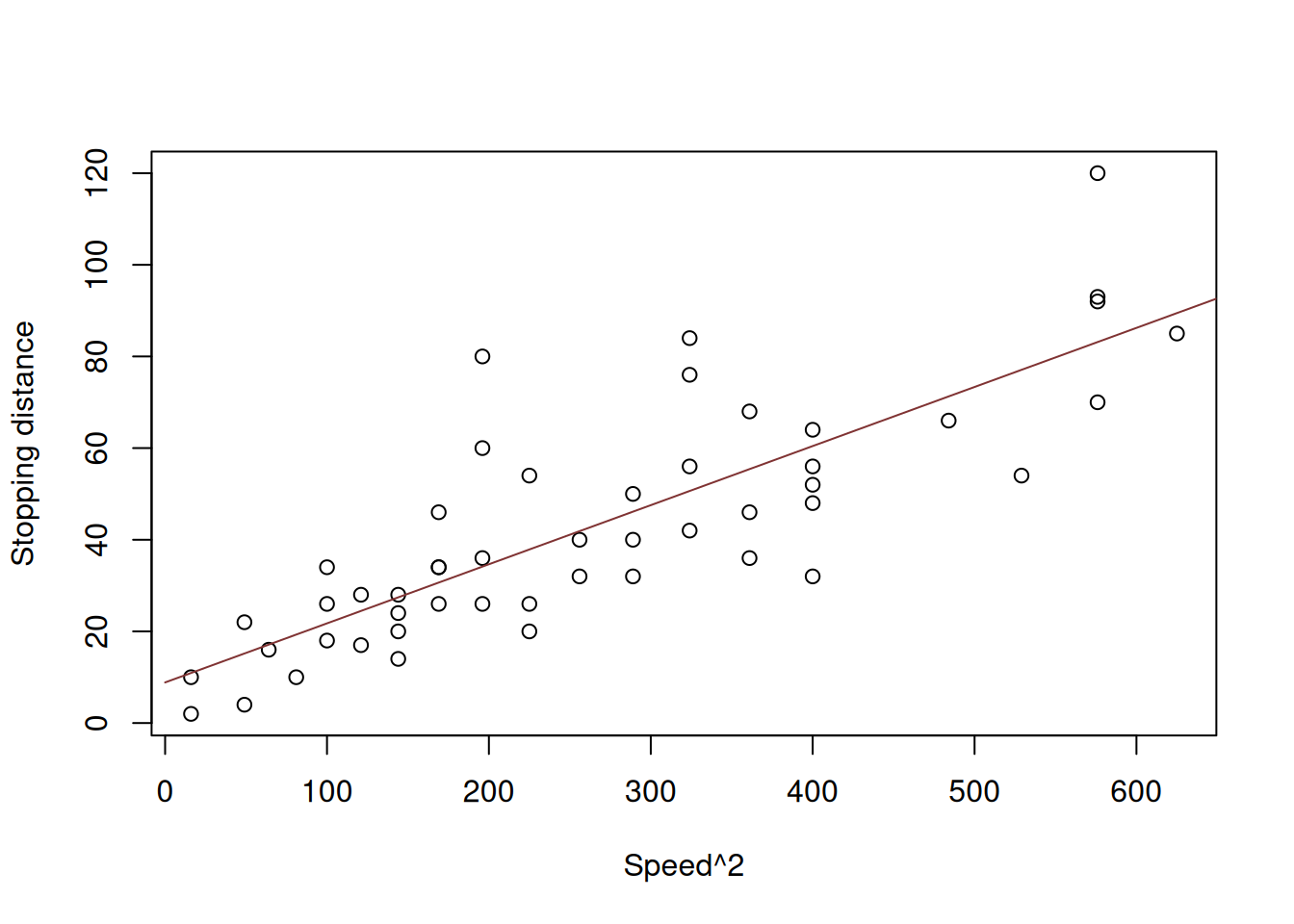
Figure 14.4: Speed squared vs stopping distance.
Figure 14.4 demonstrates the scatterplot for squared speed vs stopping distances. While we see that the relation between variables is closer to linear, the problem with variance is not resolved. If we want to estimate this model, we can use the following command in R:
Note that we use I() in the formula to tell R to square the variable - it will not do the necessary transformation otherwise. Also note that in our specific case we did not include the non-transformed speed variable, because we know that the lowest distance should be, when speed is zero. But this might not be the case in other cases, so in general instead of the formula used above we should use: y~x+I(x^2). Furthermore, if we know for sure that the intercept is not needed (i.e. we know that the distance will be zero, when speed is zero), then we can remove it and estimate the model:
## Warning: You have asked not to include intercept in the model. We will try to
## fit the model, but this is a very naughty thing to do, and we cannot guarantee
## that it will work...
alm() function will complain about the exclusion of the intercept, but it should estimate the model nonetheless. The fit of the model to the data would be similar in its shape to the one from the log-log model (see Figure 14.5).
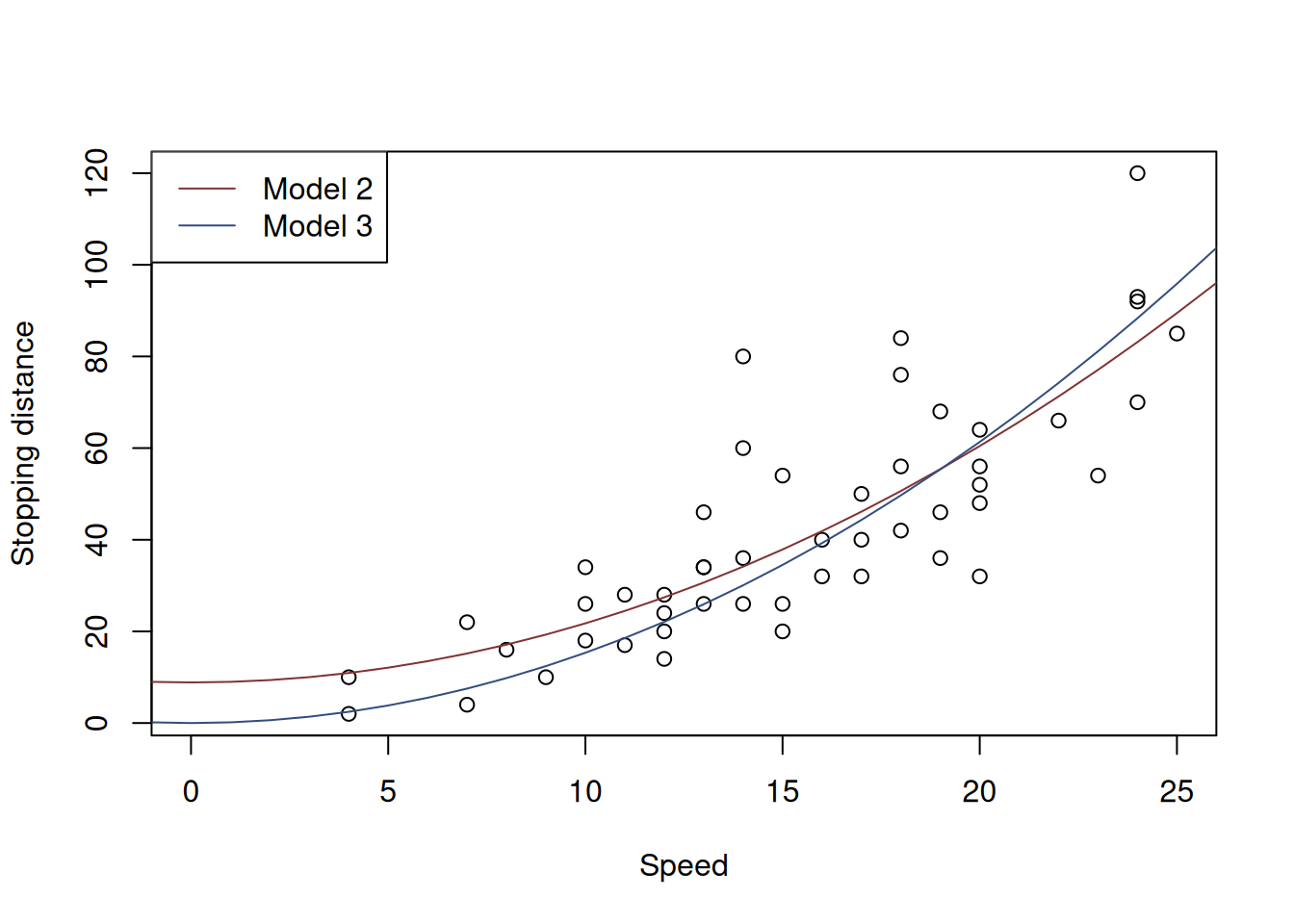
Figure 14.5: Speed squared vs stopping distance with models with speed^2.
The plot in Figure 14.5 demonstrates how the two models fit the data. The Model 2, as we see goes through the origin, which makes sense from the physical point of view. However, because of that it might fit the data worse than the Model 1 does. Still, it it better to have a more meaningful model than the one that potentially overfits the data.
Another way to introduce the squares in the model is to take square root of distance. This would potentially align better with the physical model of stopping distance (14.1): \[\begin{equation} \sqrt{distance} = \beta_0 + \beta_1 speed + \epsilon , \tag{14.5} \end{equation}\] which will be equivalent to: \[\begin{equation} distance = (\beta_0 + \beta_1 speed + \epsilon)^2 . \tag{14.6} \end{equation}\] The good news is, the error term in this model will change with the change of speed due to the interaction effect, cause by the square of the sum in (14.6). And, similar to the previous models, the parameter \(\beta_0\) might not be needed. Graphically, this transformation is present on Figure 14.6.
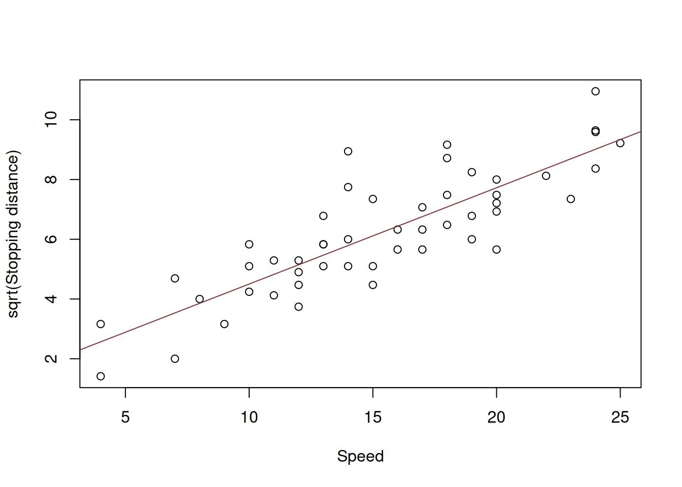
Figure 14.6: Speed vs square root of stopping distance.
As the plot in Figure 14.6 demonstrates, the relation has become linear and the variance seems to be constant, no matter what the speed is. This means that the proposed model might be more appropriate to the data than the previous ones. This is how we can estimate this model:
Similar to the Model 2 with squares, we will also consider the model without intercept on the grounds that if we capture the relation correctly, the zero speed should result in zero distance.
## Warning: You have asked not to include intercept in the model. We will try to
## fit the model, but this is a very naughty thing to do, and we cannot guarantee
## that it will work...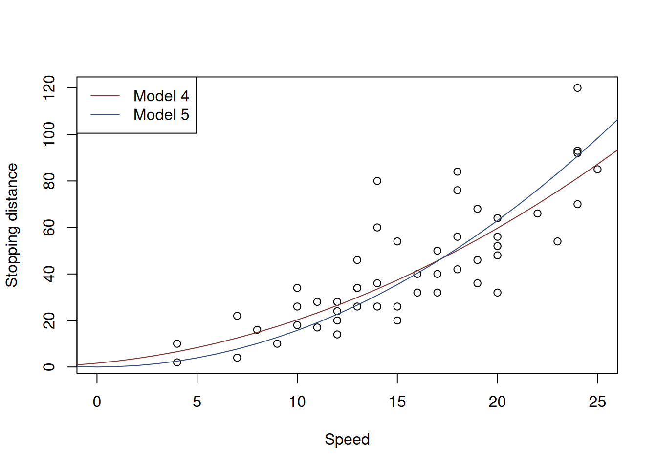
Figure 14.7: Speed squared vs stopping distance with Square Root models.
Subjectively, I would say that Model 5 is the most appropriate from all the models under consideration: it corresponds to the physical model on one hand, and has constant variance on the other one. Here is its summary:
## Response variable: sqrtdist
## Distribution used in the estimation: Normal
## Loss function used in estimation: MSE
## Coefficients:
##       Estimate Std. Error Lower 2.5% Upper 97.5%
## speed   0.3967     0.0102     0.3764      0.4171 *
##
## Error standard deviation: 1.1674
## Sample size: 50
## Number of estimated parameters: 1
## Number of degrees of freedom: 49
## Information criteria:
##      AIC     AICc      BIC     BICc
## 160.3623 160.6176 164.1863 164.6857
Its parameter contains some average information about the mass of cars and their breaking forces (this is based on the formula (14.1)). The interpretation of the parameter in this model, however, is challenging. In order to get to some crude interpretation, we need to revert to maths. Model 5 can be written as: \[\begin{equation} distance = (\beta_1 speed + \epsilon)^2 . \tag{14.7} \end{equation}\] If we take the first derivative of distance with respect to speed, we will get: \[\begin{equation} \frac{\mathrm{d}distance}{\mathrm{d}speed} = 2 (\beta_1 speed + \epsilon) , \tag{14.8} \end{equation}\] which is now closer to what we need. We can say that if speed increases by 1mph, the distance will change on average by \(2 \beta_1 speed\). But this does not explain what the meaning of \(\beta_1\) in the model is. So we take the second derivative with respect to speed: \[\begin{equation} \frac{\mathrm{d}^2 distance}{\mathrm{d}^2 speed} = 2 \beta_1 . \tag{14.9} \end{equation}\] The meaning of the second derivative is that it shows the change of change of distance with a change of change of speed by 1. This implies a tricky interpretation of the parameter. Based on the summary above, the only thing we can conclude is that when the change of speed increases by 1mph, the change of distance will increase by 0.7934 feet. An alternative interpretation would be based on the model (14.5): with the increase of speed of car by 1mph, the square roo tof stopping distance would increase by 0.3967 square root feet. Neither of these two interpretations are very helpful, but this is the best we have for the parameter \(\beta_1\) in the Model 5.