10.2 Covariance, correlation and SLR
Now that we have introduced a simple linear regression, we can take a step back to better understand some statistics related to it, which we discussed in previous chapters.
10.2.1 Covariance
Covariance is one of the most complicated things to explain to general audience. We will need to use a bit of mathematics that we introduced in Section 10.1, specifically the formula (10.6), where \(b_1\) is calculated as: \[\begin{equation*} {b}_1 = \frac{\mathrm{cov}(x,y)}{\hat{\sigma}_x^2} , \end{equation*}\] where \(\hat{\sigma}_x\) is the in-sample estimate of standard deviation. Using a simple manipulation, we can express cov\((x,y)\) as: \[\begin{equation*} \mathrm{cov}(x,y) = {b}_1 \hat{\sigma}_x \hat{\sigma}_x . \end{equation*}\] Visually, this can be represented as the areas of a rectangular shown on right pane in Figure 10.7.
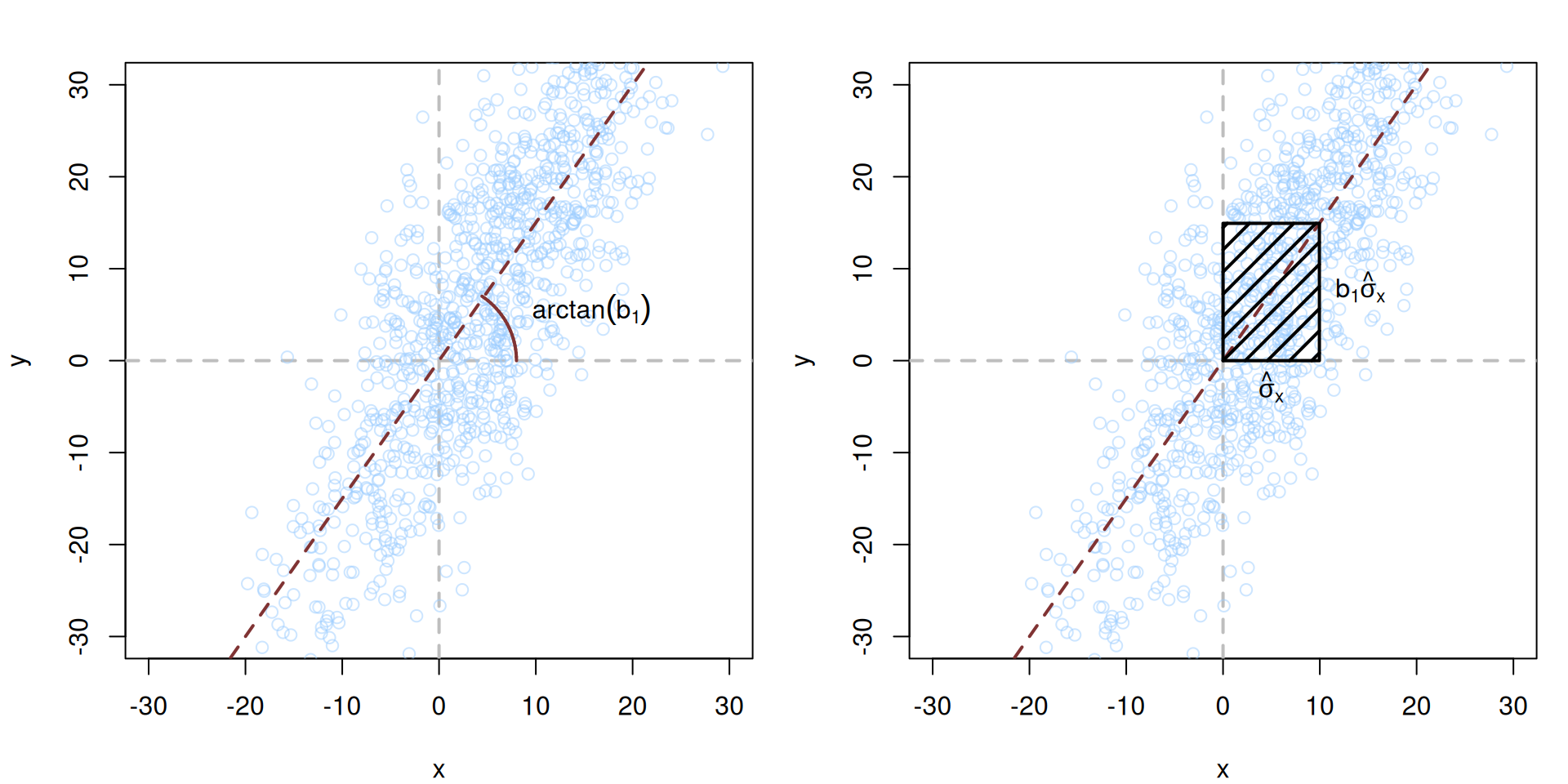
Figure 10.7: Visualisation of covariance between two random variables, \(x\) and \(y\).
In Figure 10.7, the data is centred around the means of \(x\) and \(y\). We draw a regression line with the angle \(\arctan (b_1)\) through the cloud of points (the left-hand side image). After that we draw a segment of the length \(\hat{\sigma}_x\) parallel to the x-ays (righ-hand side image). The multiplication of \(b_1\) by \(\hat{\sigma}_x\) gives the side denoted as \(b_1 \hat{\sigma}_x\) (because \(b_1\) equals to tangent of the angle of the line to the x-ays). And finally, the \(b_1 \hat{\sigma}_x \times \hat{\sigma}_x = \mathrm{cov}(x,y)\) is the area of the rectangular in the right-hand side image of Figure 10.7. The higher the standard deviation of \(x\) is, the bigger the area will be, implying that the covariance becomes larger. At the same time, for the same values of \(\hat{\sigma}_x\), the higher \(b_1\) is, the larger the area becomes, increasing the covariance as well. In this interpretation the covariance becomes equal to zero in one of the two cases: \[\begin{equation*} \begin{aligned} & {b}_1 = 0 \\ & \hat{\sigma}_x =0 , \end{aligned} \end{equation*}\] which implies that either the angle of the regression line is zero, i.e. there is no linear relation between \(x\) and \(y\), or there is no variability in the variable \(x\).
Similar visualisations can be done if the axes are swapped and the regression \(x = a_0 + a_1 y + u\) is constructed. The logic would be similar, only changing the value of the slope parameter \(b_1\) by \(a_1\) and substituting \(\hat{\sigma}_x\) with \(\hat{\sigma}_y\). Finally, in case of negative relation between the variables, the rectangular area will be drawn below the zero line and thus could be considered as being negative (although the surface of the area itself cannot be negative). Still, the logic explained for the positive case above could be transferred on the negative case as well.
10.2.2 Correlation
Another thing to discuss is the connection between the parameter \({b}_1\) and the correlation coefficient. We have already briefly mentioned that in Section 9.3, but here we can now spend more time on it. First, we could estimate two models given the pair of variable \(x\) and \(y\):
- Model (10.3) \(y_j = b_0 + b_1 x_j + e_j\);
- The inverse model \(x_j = a_0 + a_1 y_j + u_j\).
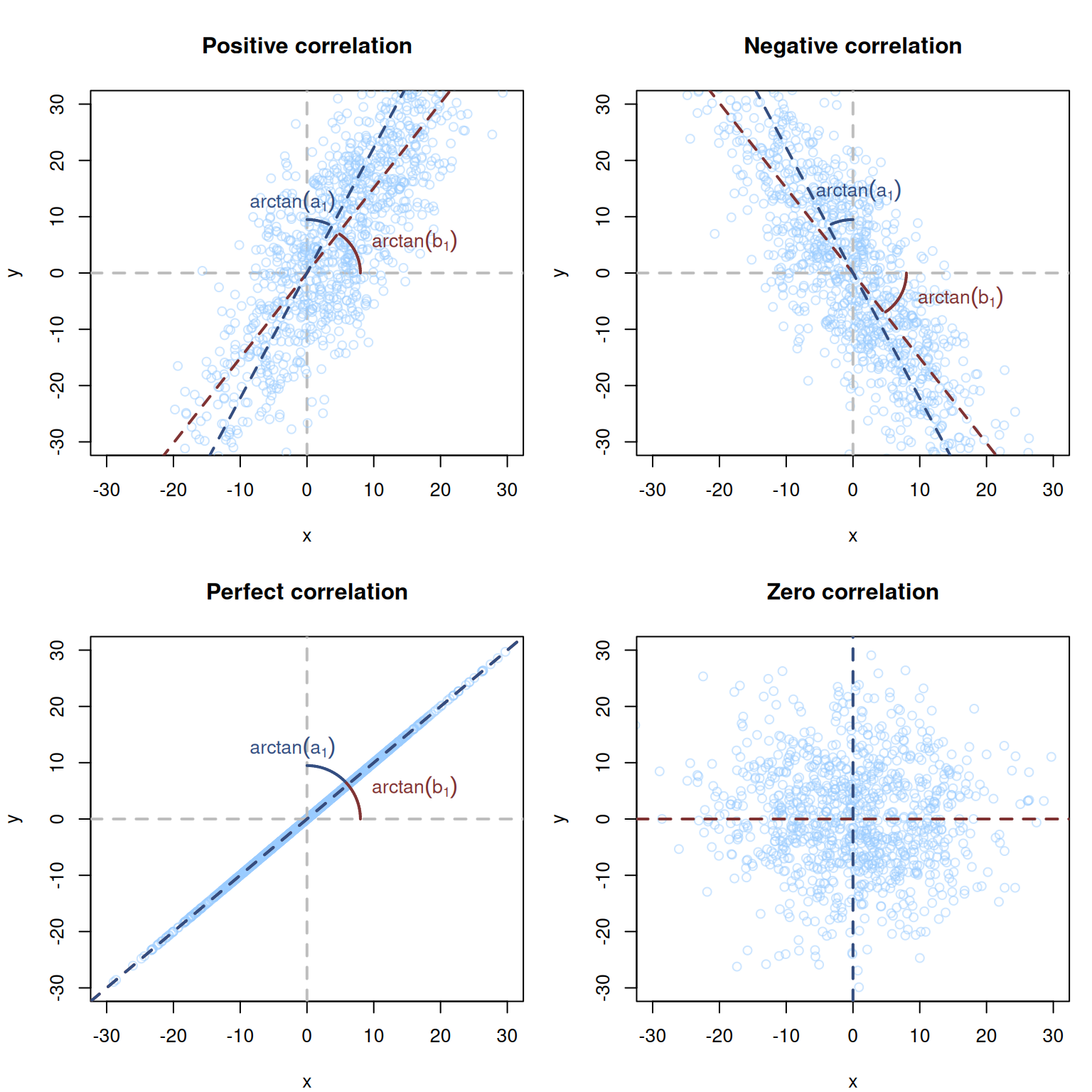
Figure 10.8: Visualisation of correlations between two random variables, \(x\) and \(y\) for four cases: positive, negative, perfect and zero correlation.
If the lines have positive slopes (as shown in the left top pane in Figure 10.8) then the resulting coefficient of correlation will be positive. If they are both negative, the correlation will be negative as well (right top pane in Figure 10.8). If the lines coincide then the product of tangents of their angles will be equal to 1 (thus we would have a perfect correlation of 1, left bottom pane in Figure 10.8). Finally, in the case, when there is no linear relation between variables, the lines will coincide with the x- and y- axes respectively, producing \(a_1=b_1=0\) and thus leading to the zero correlation coefficient (right bottom pane in Figure 10.8).
Finally, another way to look at the correlation is to consider the visualisation of covariance from Figure 10.7 and to expand it to the correlation coefficient, for which the part \(\hat{\sigma}_x \times \hat{\sigma}_y\), corresponds to the denominator in the formula (10.8), and is shown in Figure 10.9 as a red area.
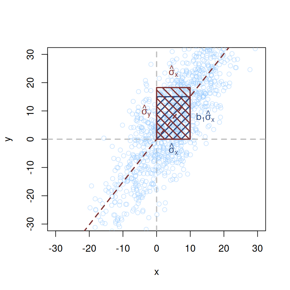
Figure 10.9: Visualisation of correlation between two random variables, \(x\) and \(y\).
The correlation in Figure 10.9, corresponds to the ratio of the two areas: blue one (covariance) to the red one (the product of standard deviations). If the areas coincide, the correlation is equal to one. This would only happen if all the observations lie on the straight line, the case for which \(\hat{\sigma}_y = b_1 \hat{\sigma}_x\). Mathematically, this can be seen if we take the variance of the response variable conditional on the slope parameter: \[\begin{equation} \mathrm{V}(y | b_1) = b_1^2 \mathrm{V}(x) + V(e), \tag{10.9} \end{equation}\] which leads to the following equality for the conditional standard deviation of \(y\): \[\begin{equation} \hat{\sigma}_y = \sqrt{b_1^2 \hat{\sigma}_x^2 + \hat{\sigma}_e^2} , \tag{10.10} \end{equation}\] where \(\hat{\sigma}_e\) is the standard deviation of the residuals. In this case, it becomes clear that the correlation is impacted by the variance of the error term \(\hat{\sigma}_e^2\). If it is equal to zero, we get the equality: \(\hat{\sigma}_y = b_1 \hat{\sigma}_x\), for which the areas in Figure 10.9 will coincide and correlation becomes equal to one. The bigger the variance of residuals is, the lower the correlation coefficient becomes. Note that the value of \(b_1\) does not impact the strength of correlation, it only regulates, whether the correlation is positive, negative or zero. Several correlation coefficients and respective rectangular areas are shown in Figure 10.10.
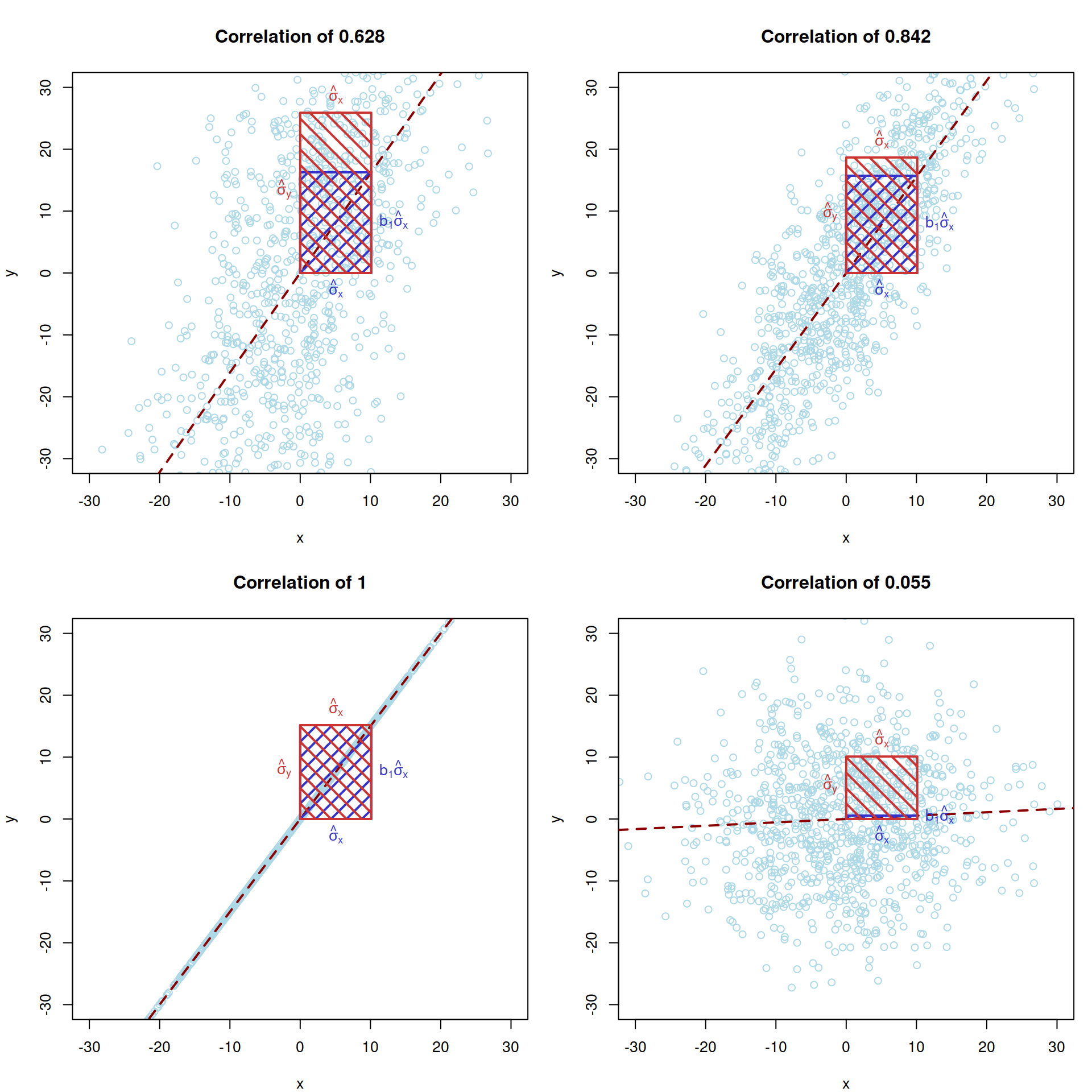
Figure 10.10: Visualisation of several correlation coefficients.