5.2 Graphical analysis
5.2.1 One categorical/discrete variable
Continuing our example with mtcars dataset, we now investigate what plots can be used for different types of data. As discussed earlier, we have two categorical variables: vs and am - and they need to be treated differently than the numerical ones. We can start by producing their barplots:
barplotVS <- barplot(table(mtcarsData$vs), xlab="Type of engine", col=17)
text(barplotVS,table(mtcarsData$vs)/2,table(mtcarsData$vs),cex=1.25)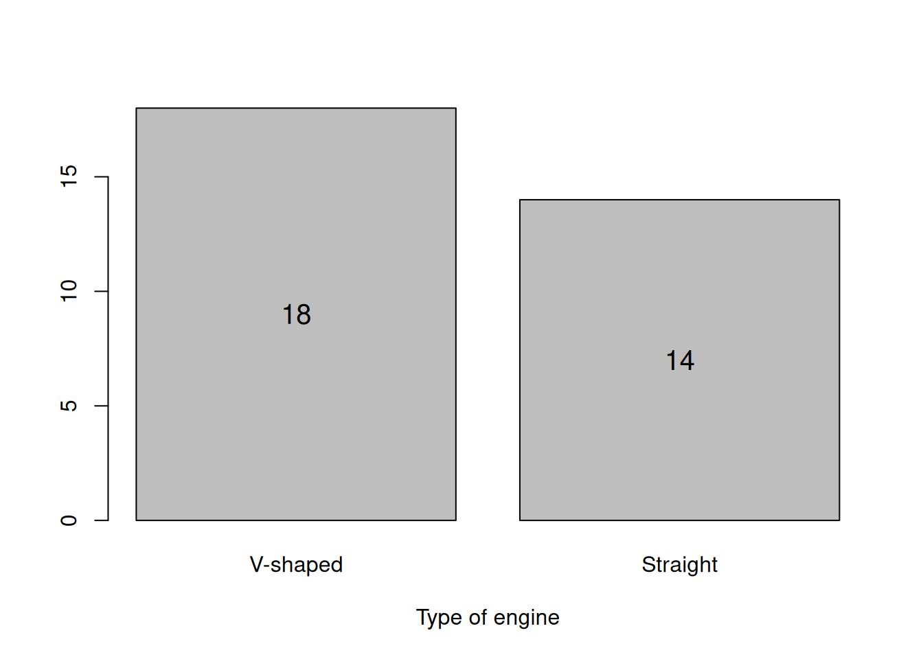
Figure 5.2: Barplot for the engine type.
This is just a graphical presentation of the contingency table we have already discussed earlier.
Remark. Histograms do not make sense in case of categorical variables, because they assume that variables are numerical and continuous (see Section 2.2) - they will split the values of a variable in the bins, based on the idea that the variable can take any of the values in each bin.
Barplots are useful when you deal with either categorical variables or integer numerical ones. Here is what we can produce in case of the integer variable cyl:
barplotCYL <- barplot(table(mtcarsData$cyl),
                      xlab="Number of cylinders", col=17)
text(barplotCYL, table(mtcarsData$cyl)/2, table(mtcarsData$cyl), cex=1.25)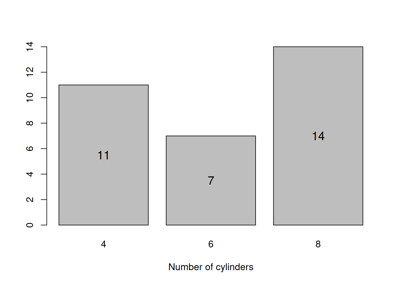
Figure 5.3: Barplot for the number of cylinders.
Figure 5.3 shows that there are three types of cars in the data: with 4, 6 and 8 cylinders. The most frequently met is the car with 8 cylinders. Judging by the plot, half of cars have not more than 6 cylinders (median is equal to 6). All of this can be deducted from the barplot. And here how the histogram would look like for cylinders:
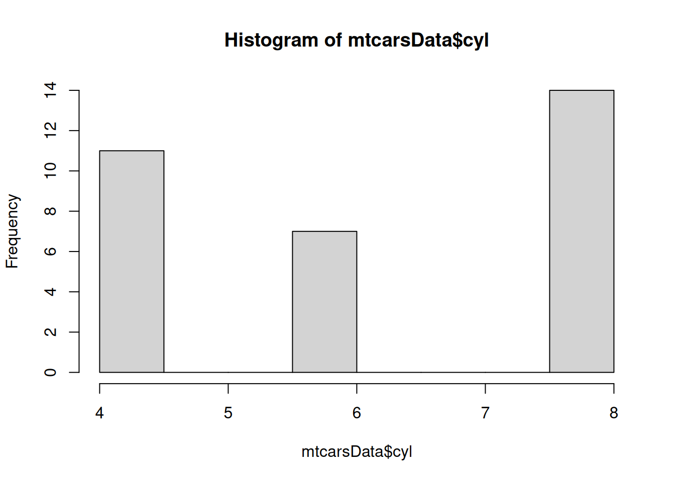
Figure 5.4: Histogram for the number of cylinders. Do not do this!
Figure 5.4 is difficult to read, because on histogram, the bars show frequency at which continuous variable appears in pre-specified bins. In our case we would conclude that the most frequently cars in the dataset are those that have 7.5 - 8 cylinders, which is wrong and misleading. In addition, this basic plot does not have a readable label for x-axis and a meaningful title (in fact, we do not need one, given that we have caption). So, always label your axis and make sure that the text on plots is easy to understand for those people who do not work with the data.
5.2.2 Two categorical/discrete variables
Coming back to categorical variables, we can construct two-dimensional plots to investigate potential relations between variables. We will first try the same barplot as above, but with vs and am variables:
barplot(table(mtcarsData$vs,mtcarsData$am),
        xlab="Type of transmission", legend.text=levels(mtcarsData$vs))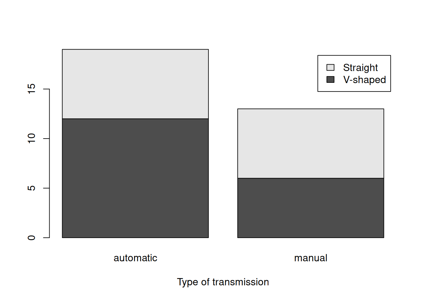
Figure 5.5: Barplot for the type of engine and transmission.
Figure 5.5 provides some information about the distribution of type of engine and transmission. For example, we can say that the most often met car in the dataset is the one with automatic transmission and V-shaped engine. However, it is not possible to say much about the relation between the two variables based on this plot. So, there is an alternative presentation, which uses the heat map (tableplot() from greybox):
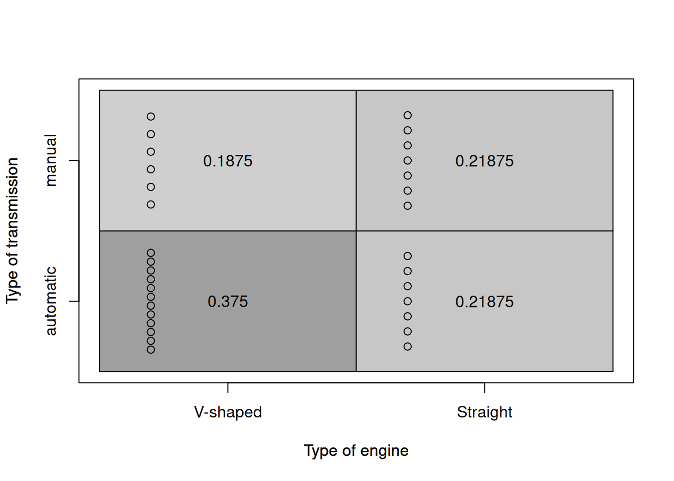
Figure 5.6: Heat map for the type of engine and transmission.
The idea of this plot is that the darkness of areas shows the frequency of occurrence of each specific value. This message is duplicated by the number of dots in the plot (the more dots there are, the more observations there are in that specific area). The numbers inside the box show the proportions for each answer. So, we can conclude (again), that automatic transmission with V-shaped engine is met in 37.5% of cases. On the other hand, the least frequent type of car is the one with V-shaped engine and manual transmission. There might be some tendency in the dataset: the engine and transmission might be related (v-shaped with automatic vs Straigh with manual) - but it is not very well pronounced. The same table plot can be used for the analysis of relations between integer variables (and categorical). Here, for example, the plot between the number of cylinders and the type of engine:
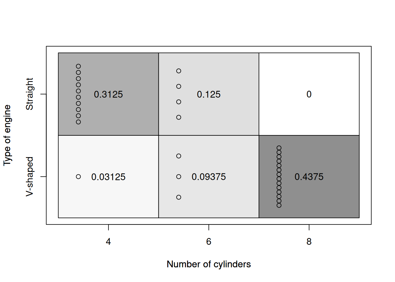
Figure 5.7: Heat map for the number of cylinders and the type of engine.
Figure 5.7 allows making more solid conclusions about the relation between the two variables: we see that with the increase of the number of cylinders, the cars tend to switch from Straight to the V-shaped engines. This has an explanation: the engines with more cylinders need to have a different geometry to fit them all, and the V shape is more suitable for them. The table plot shows clearly this relation between the two variables.
5.2.3 One numerical continuous variable
Next, we can analyse the numerical continuous variables. We can start with the basic histogram:
hist(mtcarsData$wt, xlab="Weight", main="", probability=TRUE,
     col=17)
lines(density(mtcarsData$wt), col=2, lwd=2)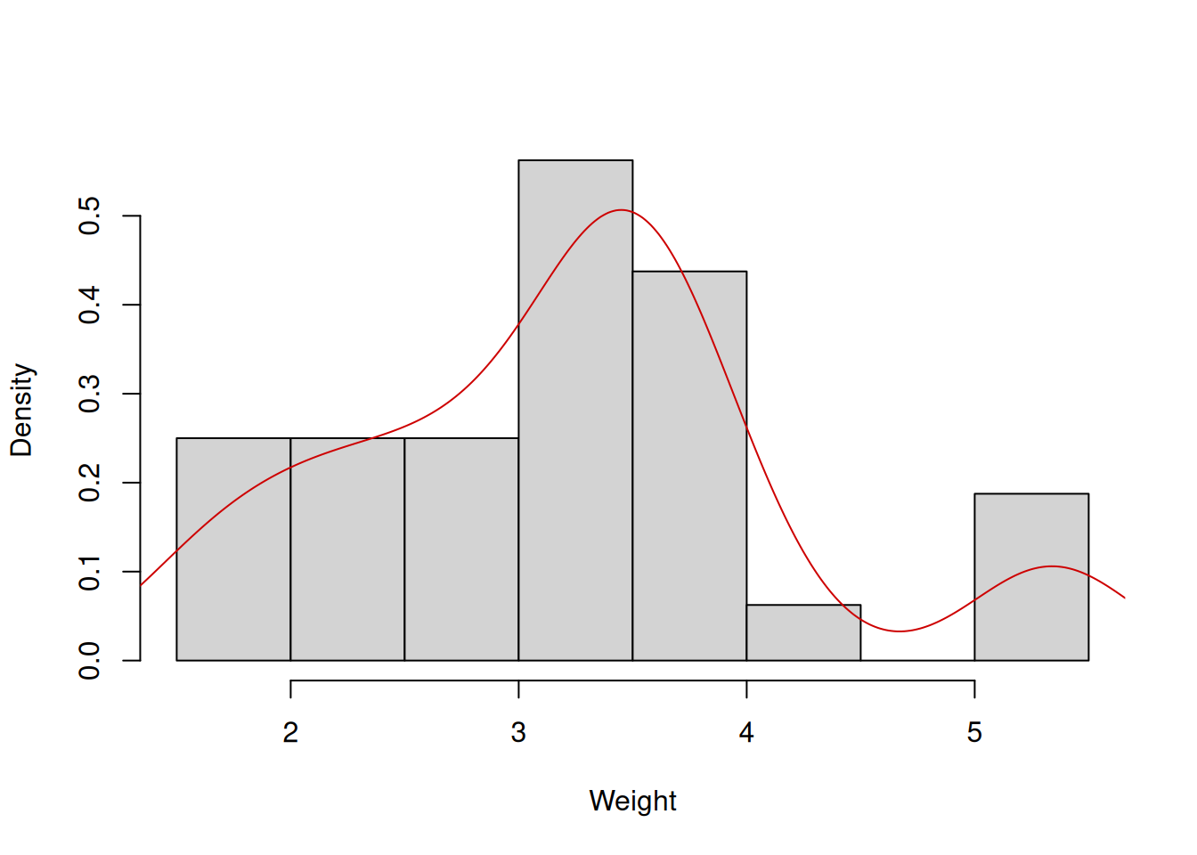
Figure 5.8: Distribution of the weights of cars.
The histogram 5.8 shows that there is a slight skewness in the data: the cars with weight from 3 to 4 thousands pounds are met more often than the cars with more than 5. The left tail of this distribution is slightly longer than the right one. Note that I have produced the probabilities on the y-axis of the plot in order to add the density curve, which smooths out the frequencies and shows how the distribution looks like.
An alternative presentation of the histogram is the boxplot, which graphically presents quantiles of distribution:
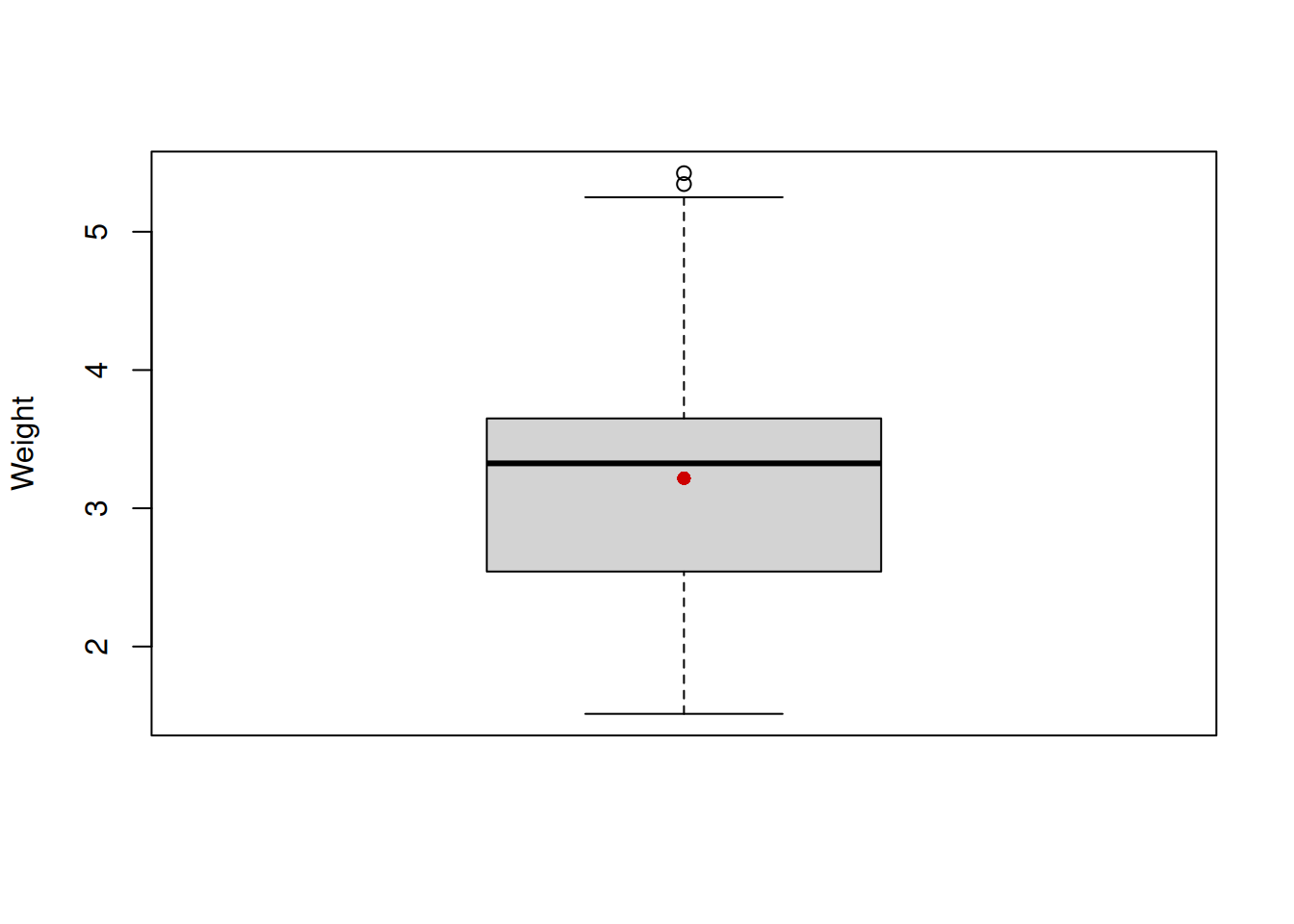
Figure 5.9: Boxplot of the variable weight.
This plot has the box in the middle, the whiskers on the sides, points at the top and the red point at the centre. The box shows 1st, 2nd and 3rd quartiles of distribution, thus the black line in the middle is the median. The distance between the 1st and the 3rd quartiles is called “Interquartile range” (IQR) and is used for the calculation of the interval (1st / 3rd quartile \(\pm 1.5 \times\)IQR), which corresponds roughly to the 99.3% interval (read more about this in Section ??) from Normal distribution and is graphically drawn as the furthest observation in the interval. So, the lower whisker on our plot corresponds to the minimum value in the data, which is still in the interval, while the upper whisker corresponds to the bound of the interval. All the observations that lie beyond the interval are marked as potential outliers. Note that this does not mean that the values are indeed outliers, they just lie outside the 99.3% interval of Normal distribution. Finally, the red dot was added by me to show where the mean is. It is lower than median, this implies that there is a slight skewness in the distribution of weight.
There is also a way for producing the plots that would combine elements of histogram, density curve and boxplot. There is a plot called “violin plot”. We will use vioplot() function from vioplot package in order to produce them:
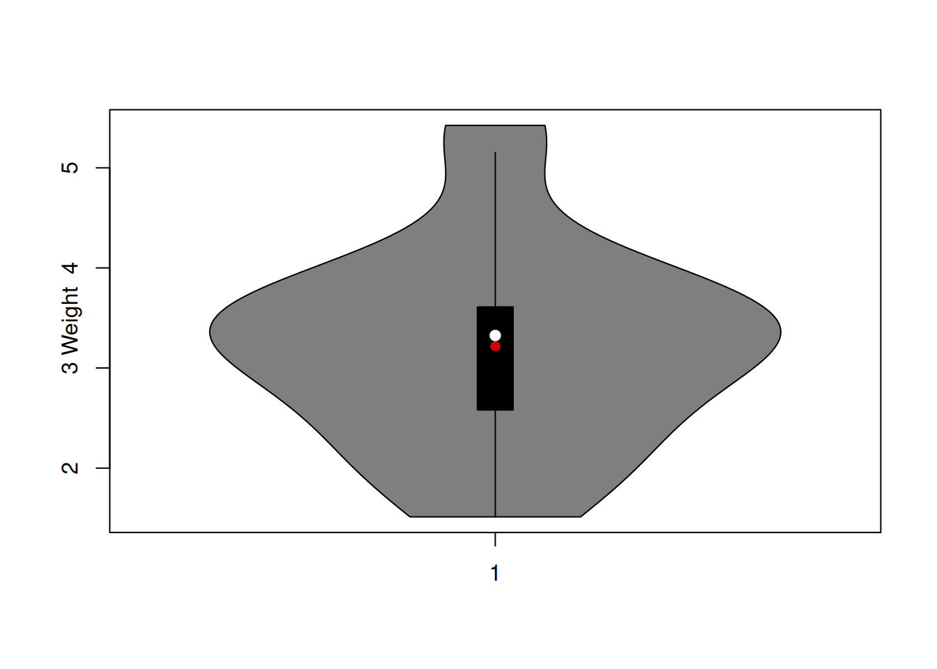
Figure 5.10: Violin plot together with boxplot of the variable weight.
Figure 5.10 unites the boxplot and the density curve from the plots above, providing not only information about the quantiles, but also about the shape of the distribution.
Finally, if we want to compare the distribution of a variable with a known theoretical distribution, we can produce the QQ-plot. Here how it looks for Normal distribution:
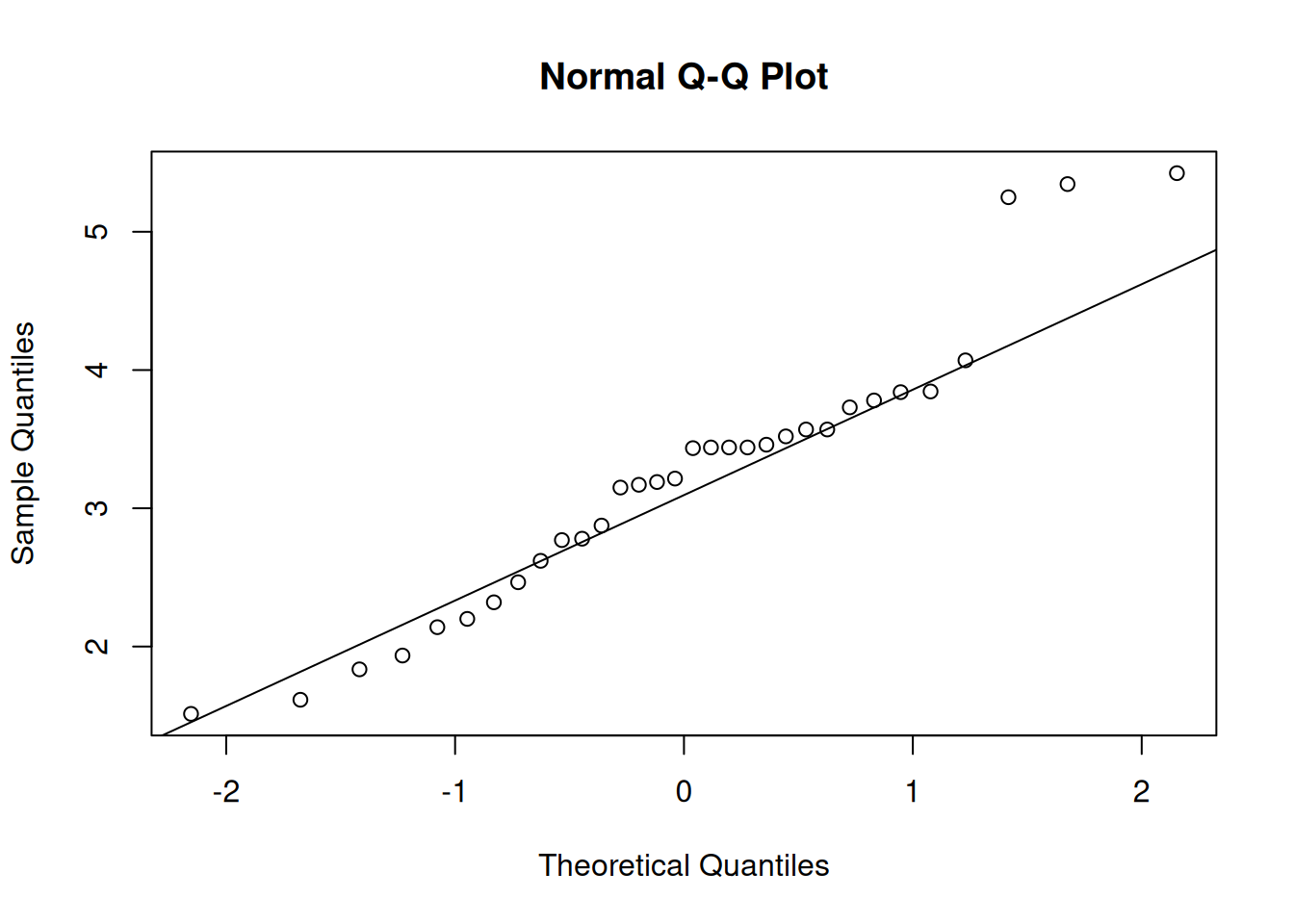
Figure 5.11: QQ plot of Normal distribution for variable weight.
The idea of the plot on Figure 5.11 is to compare theoretical quantiles with the empirical ones. If the variable would follow the specific distribution, then all the points would lie on the solid line. In our case, they do not: there are points in the right tail that are very far from the line - so we would conclude that the distribution of weight does not look Normal.
5.2.4 Two continuous numerical variables
So far, we have discussed the univariate analysis of numerical variables, but we can also produce plots showing potential relations between them. We start with the classical scatterplot:
plot(mtcarsData$wt, mtcarsData$mpg, xlab="Weight", ylab="Mileage")
lines(lowess(mtcarsData$wt, mtcarsData$mpg), col=2, lwd=2)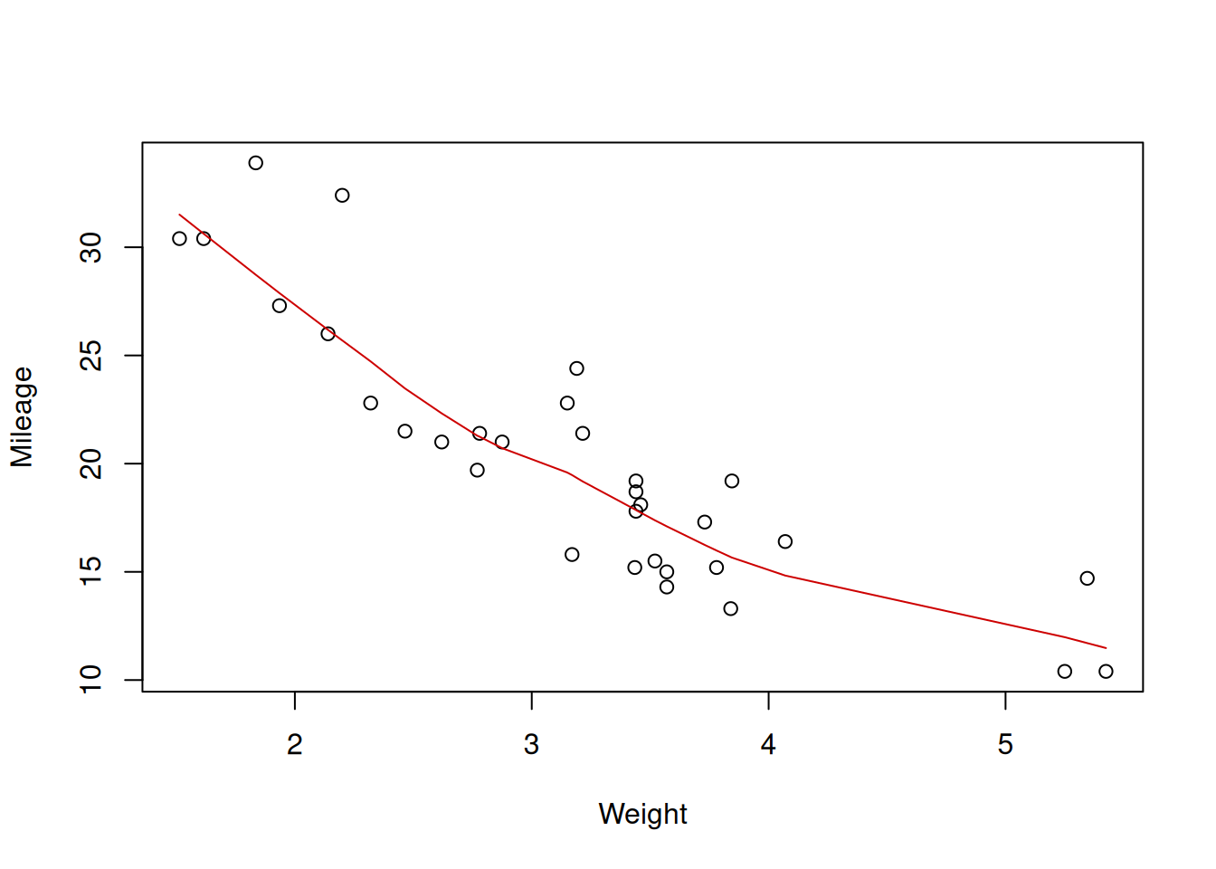
Figure 5.12: Scatterplot diagram between weight and mileage.
The plot on Figure 5.12 shows the observations that have specific weight and mileage. Based on this, we can see if there is a relation between variables or not and what sort of relation this is. In order to simplify analysis, I have added the lowess line to the plot. It smooths the relation between variables, drawing the smooth line through the points and helps in understanding the existing relations in the data. Judging by Figure 5.12, there is a negative, slightly non-linear relation between the variables: the mileage decreases with reduced speed, when weight of a car increases. This relation makes sense, because heavier cars will consume more fuel and thus drive less on a gallon of petrol.
5.2.5 A mixture of variables
We could construct similar plots for all the other numerical variables, but not all plots would be helpful. For example, a plot of mileage versus number of forward gears would be very difficult to read (see Figure 5.13).
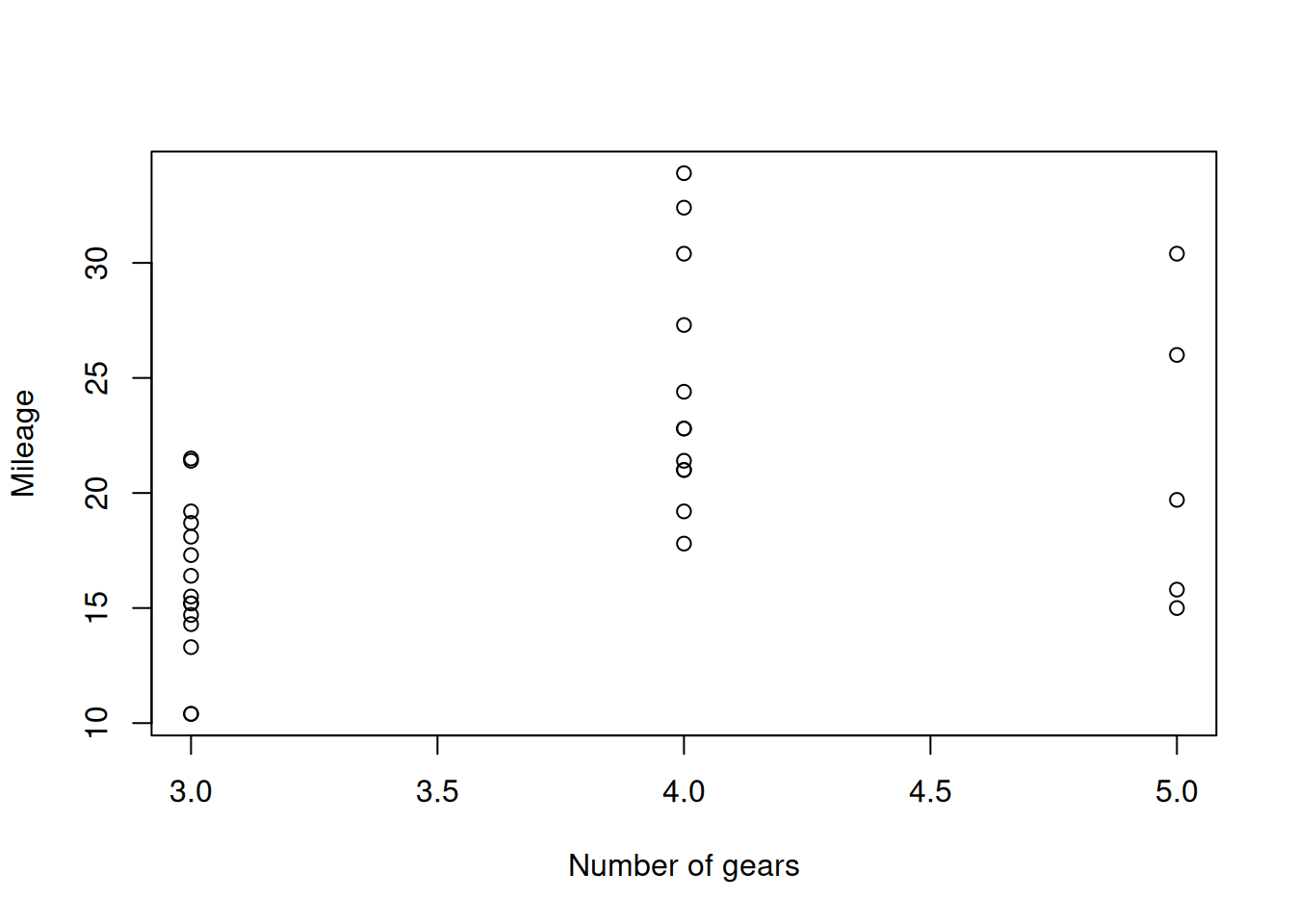
Figure 5.13: Scatterplot diagram between weight and mileage.
This is because one of the variables is integer and takes only a handful of values. In this case, a boxplot or a violin plot would be more useful:
boxplot(mpg~gear, mtcarsData, xlab="Number of gears", ylab="Mileage")
points(tapply(mtcarsData$mpg, mtcarsData$gear, mean), col=2, pch=16)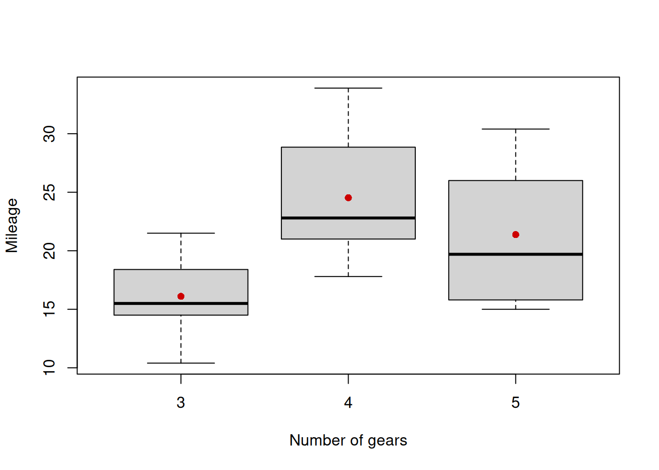
Figure 5.14: Boxplot of mileage vs number of gears.
The plot on Figure 5.14 is more informative than the one on Figure 5.13: it shows how the distribution of mileage changes with the increase of the numeric variable number of gears. We can also see that the mean value first increases and then goes down slightly. I do not have any good explanation of this phenomenon, but it might be related with how efficient the cars become with the increase fo the number of gears, or this could happen due to some latent, unobserved factors. So, the data tells us that there is a non-linear relation between number of gears and mileage.
Similarly, we can produce violin plots for the same data using the following code:
vioplot(mpg~gear, mtcarsData, xlab="Number of gears", ylab="Mileage",
        col=17, rectCol=16)
points(tapply(mtcarsData$mpg, mtcarsData$gear, mean), col=2, pch=16)
Finally, using exactly the same idea with boxplots / violin plots, we can analyse relations between categorical and numerical variables. Figure 5.15 shows the relation between transmission type and mileage. We can conclude that the cars with manual transmission tend to have a higher mileage than the ones with the automatic one in our dataset.
vioplot(mpg~am, mtcarsData, xlab="Transmission type", ylab="Mileage",
        col=17, rectCol=16)
points(tapply(mtcarsData$mpg, mtcarsData$am, mean), col=2, pch=16)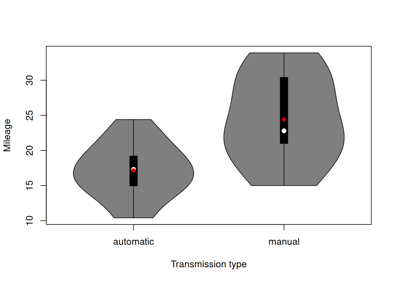
Figure 5.15: Violin plot of mileage vs transmission type.
5.2.6 Plot for several variables
Finally, producing plots one by one might be a tedious and challenging task, so it is good to have some instruments for producing several of them together. The plot() method will produce scatterplot matrix for numerical variables, but does not deal well with integer and categorical variables:
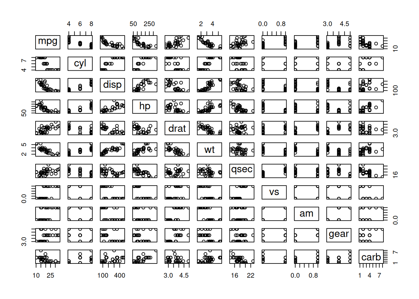
Figure 5.16: Scatterplot matrix for the mtcars dataset.
Figure 5.16 is informative for the variables mpg, cyl, disp, hp, drat, qsec and carb, but is difficult to read for the others. In order to address this issue, we can use the spread() function from greybox, which will detect types of variables and produce the necessary plots automatically:
# Amend the palette. This is just to show how to use it
# This palette is in red colours
palette(c(rgb(0.5,0.2,0.2,0.5), rgb(0.5,0.2,0.2,1), rgb(0.9,0.6,0.6,0.5)))
# Call the function
spread(mtcarsData, lowess=TRUE)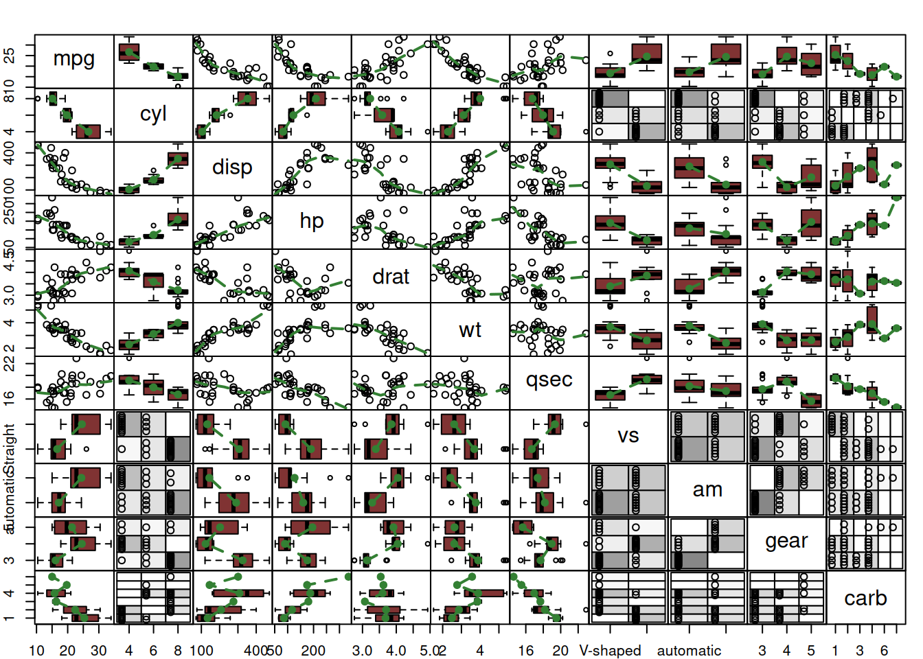
Figure 5.17: Spread plot for the mtcars dataset.
The plot on Figure 5.17 is the collection of the plots discussed above, so I will not stop on explaining what it shows.
As a final word for this section, when analysing data, it is critically important not to just describe what we see, but also explain why a result or a relationship is meaningful, otherwise this becomes an exercise of stating the obvious which does not have any value. So, for example, concluding based on Figure 5.17 that the mileage has a negative relation with displacement is not enough. If you want to analyse the data properly, you need to explain that this relation is meaningful, because with the increase of the size of engine, the fuel consumption will increase as well, and as a result the mileage will go down. Furthermore, the relation is non-linear because the change in decrease will slow down with cars with bigger engines. Inevitably, the car with a gigantic engine will be able to travel a short distance on a gallon of fuel - the mileage will not become negative, so the non-linearity is not an artefact of the data, but an existing phenomenon.