This book is in Open Review. I want your feedback to make the book better for you and other readers. To add your annotation, select some text and then click the on the pop-up menu. To see the annotations of others, click the button in the upper right hand corner of the page

9.3 Numerical scale

Finally we come to the discussion of relations between variables measured in numerical scales. The most famous measure in this category is the Pearson’s correlation coefficient, which population value is: \[\begin{equation} \rho_{x,y} = \frac{\sigma_{x,y}}{\sigma_x \sigma_y}, \tag{9.9} \end{equation}\] where \(\sigma_{x,y}\) is the covariance between variables \(x\) and \(y\) (see discussions in Sections 5.1 and 10.2), while \(\sigma_x\) and \(\sigma_y\) are standard deviations of these variables. Typically, we do not know the population values, so this coefficient can be estimated in sample via: \[\begin{equation} r_{x,y} = \frac{\mathrm{cov}(x,y)}{\sqrt{V(x)V(y)}}, \tag{9.10} \end{equation}\] where all the values from (9.9) are substituted by their in-sample estimates. This coefficient measures the strength of linear relation between variables and lies between -1 and 1, where the boundary values correspond to perfect linear relation and 0 implies that there is no linear relation between the variables. In some textbooks the authors claim that this coefficient relies on Normal distribution of variables, but nothing in the formula assumes that. It was originally derived based on the simple linear regression (see Section 10) and its rough idea is to get information about the angle of the straight line drawn on the scatterplot. It might be easier to explain this on an example:

plot(mtcarsData$disp,mtcarsData$mpg,
     xlab="Displacement",ylab="Mileage")
abline(lm(mpg~disp,mtcarsData),col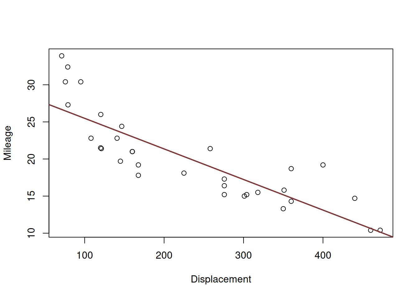="red")

Figure 9.2: Scatterplot for dispalcement vs mileage variables in mtcars dataset

Figure 9.2 shows the scatterplot between the two variables and also has the straight line, going through the cloud of points. The closer the points are to the line, the stronger the linear relation between the two variables is. The line corresponds to the formula \(\hat{y}=a_0+a_1 x\), where \(x\) is the displacement and \(\hat{y}\) is the line value for the Mileage. The same relation can be presented if we swap the axes and draw the line \(\hat{x}=b_0+b_1 y\):

plot(mtcarsData$mpg,mtcarsData$disp,
     xlab="Mileage",ylab="Displacement")
abline(lm(disp~mpg,mtcarsData),col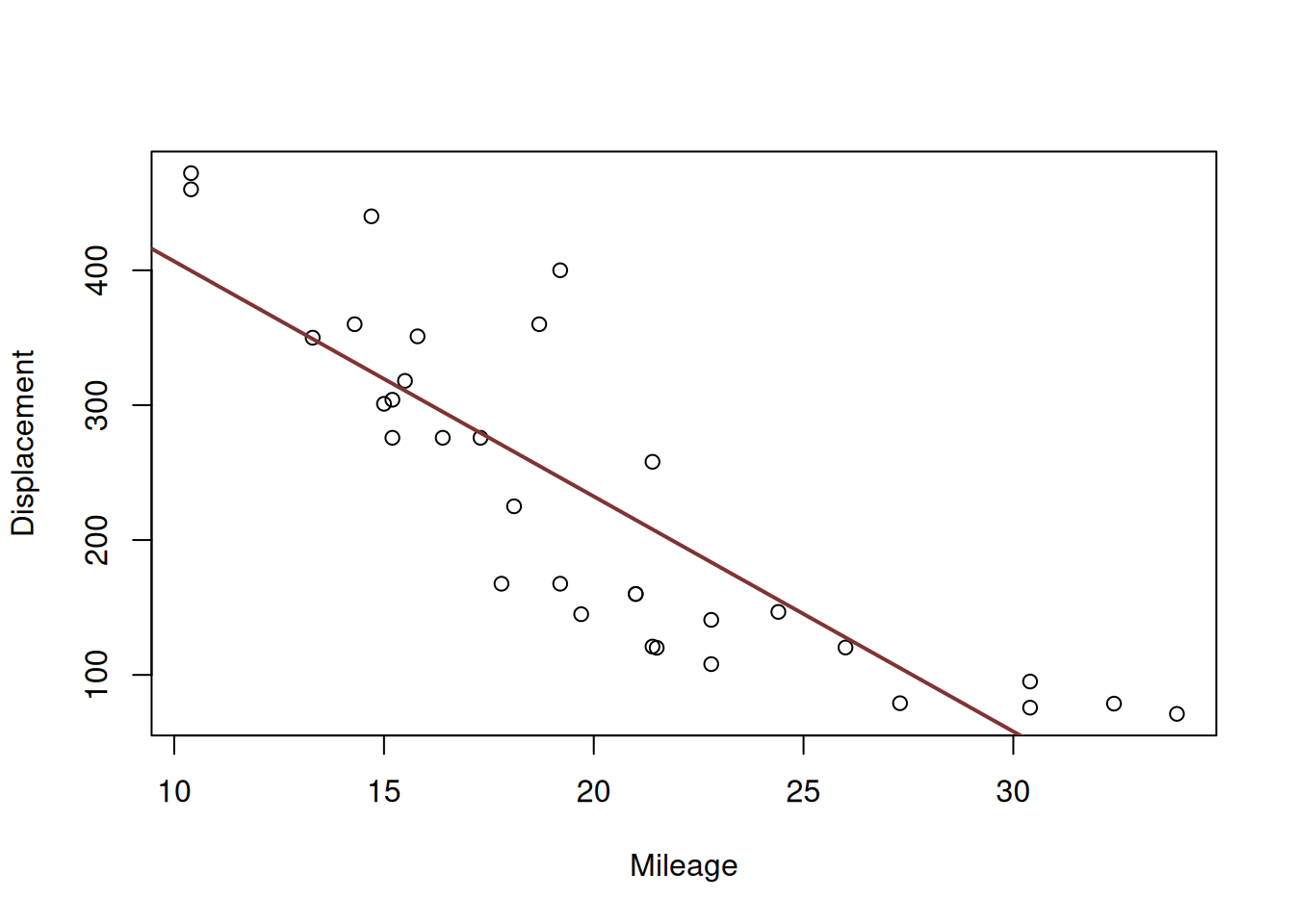="red")

Figure 9.3: Scatterplot for mileage vs dispalcement

The slopes for the two lines will in general differ, and will only coincide if the two variables have functional relations (all the point lie on the line). Based on this property, the correlation coefficient was originally constructed, as a geometric mean of the two parameters of slopes: \(r_{x,y}=\sqrt{a_1 b_1}\). We will come back to this specific formula later in Section 10. But this idea provides an explanation why the correlation coefficient measures the strength of linear relation. For the two variables of interest it will be:

cor(mtcarsData$mpg,mtcarsData$disp)

## [1] -0.8475514

Which shows strong negative linear relation between the displacement and mileage. This makes sense, because in general the cars with bigger engines will have bigger consumption and thus will make less miles per gallon of fuel. The more detailed information about the correlation is provided by the cor.test() function:

cor.test(mtcarsData$mpg,mtcarsData$disp)

## 
##  Pearson's product-moment correlation
## 
## data:  mtcarsData$mpg and mtcarsData$disp
## t = -8.7472, df = 30, p-value = 9.38e-10
## alternative hypothesis: true correlation is not equal to 0
## 95 percent confidence interval:
##  -0.9233594 -0.7081376
## sample estimates:
##        cor 
## -0.8475514

In addition to the value, we now have results of the hypothesis testing (where null hypothesis is \(\rho_{x,y}=0\)) and the confidence interval for the parameter. Given that the value of the parameter is close to its bound, we could conclude that the linear relation between the two variables is strong and statistically significant on 1% level.

Note that the value of correlation coefficient only depends on the distance of points from the straight line, it does not depend on the slope (excluding case, when slope is equal to zero and thus the coefficient is equal to zero as well). So the following two cases will have exactly the same correlation coefficients:

error <- rnorm(100,0,10)
x <- c(1:100)
y1 <- 10+0.5*x+0.5*error
y2 <- 2+1.5*x+1.5*error
# Produce the plots
par(mfcol=c(1,2))
plot(x,y1,ylim=c(0,200))
abline(lm(y1~x),col="red")
text(30,150,paste0("r=",round(cor(x,y1),5)))
plot(x,y2,ylim=c(0,200))
abline(lm(y2~x),col="red")
text(30,150,paste0("r=",round(cor(x,y2),5)))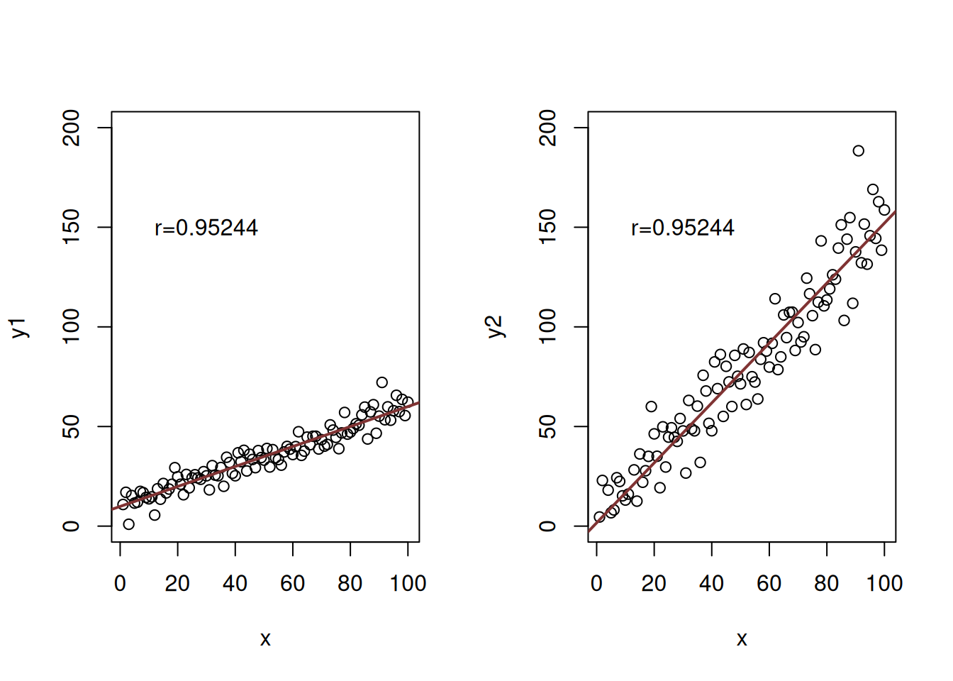

Figure 9.4: Example of relations with exactly the same correlations, but different slopes.

There are other examples of cases, when correlation coefficient would be misleading or not provide the necessary information. One of the canonical examples is the Anscombe’s quartet (Wikipedia, 2021), which shows very different types of relations, for which the Pearson’s correlation coefficient would be exactly the same. An important lesson from this is to always do graphical analysis (see Section 5.2) of your data, when possible - this way misleading situations can be avoided.

Coming back to the scatterplot in Figure 9.2, it demonstrates some non-linearity in the relation between the two variables. So, it would make sense to have a different measure that could take it into account. This is where Spearman’s correlation coefficient becomes useful. It is calculated using exactly the same formula (9.10), but applied to the data in ranks. By using ranks, we loose information about the natural zero and distances between values of the variable, but at the same time we linearise possible non-linear relations. So, Spearman’s coefficient shows the strength of monotonic relation between the two variables:

cor.test(mtcarsData$mpg,mtcarsData$disp,
         method="spearman")

## Warning in cor.test.default(mtcarsData$mpg, mtcarsData$disp, method =
## "spearman"): Cannot compute exact p-value with ties

## 
##  Spearman's rank correlation rho
## 
## data:  mtcarsData$mpg and mtcarsData$disp
## S = 10415, p-value = 6.37e-13
## alternative hypothesis: true rho is not equal to 0
## sample estimates:
##        rho 
## -0.9088824

We can notice that the value of the Spearman’s coefficient in our case is higher than the value of the Pearson’s correlation, which implies that there is indeed non-linear relation between variables. The two variables have a strong monotonic relation, which makes sense for the reasons discussed earlier. The non-linearity makes sense as well because the car with super powerful engines would still be able to do several miles on a gallon of fuel, no matter what. The relation will never be zero or even negative.

Note that while Spearman’s correlation will tell you something about monotonic relations, it will fail to capture all other non-linear relations between variables. For example, in the following case the true relation is trigonometric:

x <- c(1:100)
y <- sin(x)
plot(x,y,type="l")

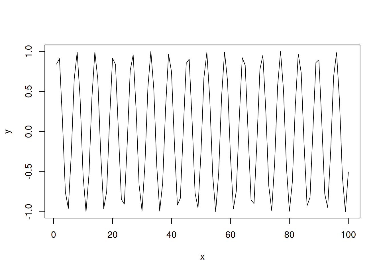
But neither Pearson’s nor Spearman’s coefficients will be able to capture it:

cor(x,y)

## [1] -0.04806497

cor(x,y,method="spearman")

## [1] -0.04649265

In order to correctly diagnose such non-linear relation, either one or both variables need to be transformed to linearise the relation. In our case this implies measuring the relation between \(y\) and \(\sin(x)\) instead of \(y\) and \(x\):

cor(sin(x),y)

## [1] 1

References

• Wikipedia, 2021. Anscombe’s quartet. https://en.wikipedia.org/wiki/Anscombe%27s_quartet (version: 2021-06-23)