5.1 Numerical analysis
In this section we will use the classical mtcars dataset from datasets package for R. It contains 32 observations with 11 variables. While all the variables are numerical, some of them are in fact categorical variables encoded as binary ones. We can check the description of the dataset in R:
Judging by the explanation in the R documentation, the following variables are categorical:
- vs - Engine (0 = V-shaped, 1 = straight),
- am - Transmission (0 = automatic, 1 = manual).
In addition, the following variables are integer numeric ones:
- cyl - Number of cylinders,
- hp - Gross horsepower,
- gear - Number of forward gears,
- carb - Number of carburettors.
All the other variables are continuous numeric.
Taking this into account, we will create a data frame, encoding the categorical variables as factors for further analysis:
mtcarsData <- data.frame(mtcars)
mtcarsData$vs <- factor(mtcarsData$vs,levels=c(0,1),labels=c("V-shaped","Straight"))
mtcarsData$am <- factor(mtcarsData$am,levels=c(0,1),labels=c("automatic","manual"))
Given that we only have two options in those variables, it is not compulsory to do this encoding, but it will help us in the further analysis.
We can start with the basic summary statistics. We remember from the scales of information (Section 1.2) that the nominal variables can be analysed only via frequencies, so this is what we can produce for them:
##
## V-shaped Straight
## 18 14##
## automatic manual
## 19 13These tables are called contingency tables, they show the frequency of appearance of values of variables. Based on this, we can conclude that the cars with V-shaped engine are met more often in the dataset than the cars with the Straight one. In addition, the automatic transmission prevails in the data. The related statistics which is useful for analysis of categorical variables is called mode. It shows which of the values happens most often in the data. Judging by the frequencies above, we can conclude that the mode for the first variable is the value “V-shaped”.
All of this is purely descriptive information, which does not provide us much. We could probably get more information if we analysed the contingency table based on these two variables:
##
##            automatic manual
##   V-shaped        12      6
##   Straight         7      7
For now, we can only conclude that the cars with V-shaped engine and automatic transmission are met more often than the other cars in the dataset.
Next, we can look at the numerical variables. As we recall from Section 1.2, this scale supports all operations, so we can use quantiles, mean, standard deviation etc. Here how we can analyse, for example, the variable mpg:
##     mean
## 20.09062## 0% 25% 50% 75% 100%
## 10.400 15.425 19.200 22.800 33.900## median
## 19.2The output above produces:
- Mean - the average value of mpg in the dataset, \(\bar{y}=\frac{1}{n}\sum_{j=1}^n y_j\).
- Quantiles - the values that show, below which values the respective proportions of the dataset lie. For example, 25% of observations have mpg less than 15.425. The 25%, 50% and 75% quantiles are also called 1st, 2nd and 3rd quartiles respectively.
- Median, which splits the sample in two halves. It corresponds to the 50% quantile.
If median is greater than mean, then this typically means that the distribution of the variable is skewed (it has some rare observations that have large values).
Making a step back, we also need to mention the variance, which shows the overall variability of the variable around its mean: \[\begin{equation} \mathrm{V}(y)= \frac{1}{n-1}\sum_{j=1}^n (y_j - \bar{y})^2 . \tag{5.1} \end{equation}\] Note that the division in (5.1) is done by \(n-1\), and not by \(n\). This is done in order to correct the value for the in-sample bias (we will discuss this in Subsection 6.4.1). The alternative formula for the variance can be derived by opening the brackets and regrouping the elements to obtain: \[\begin{equation} \mathrm{V}(y)= \mathrm{E}(y^2) - \mathrm{E}(y)^2. \tag{5.2} \end{equation}\] This form sometimes becomes useful for some derivations. The value of the variance itself does not tell us much about the variability, but having it allows calculating other more advanced measures. Typically the square root of variance is used in inferences, because it is measured in the same scale as the original data. It is called standard deviation: \[\begin{equation} \hat{\sigma} = \sqrt{\mathrm{V}(y)} , \tag{5.3} \end{equation}\] it has the same scale as the variable \(y_j\). In our example, both can be obtained via:
## [1] 36.3241## [1] 6.026948Visually, standard deviation can be represented as a straight line, depicting the overall variability of the data (Figure 5.1).
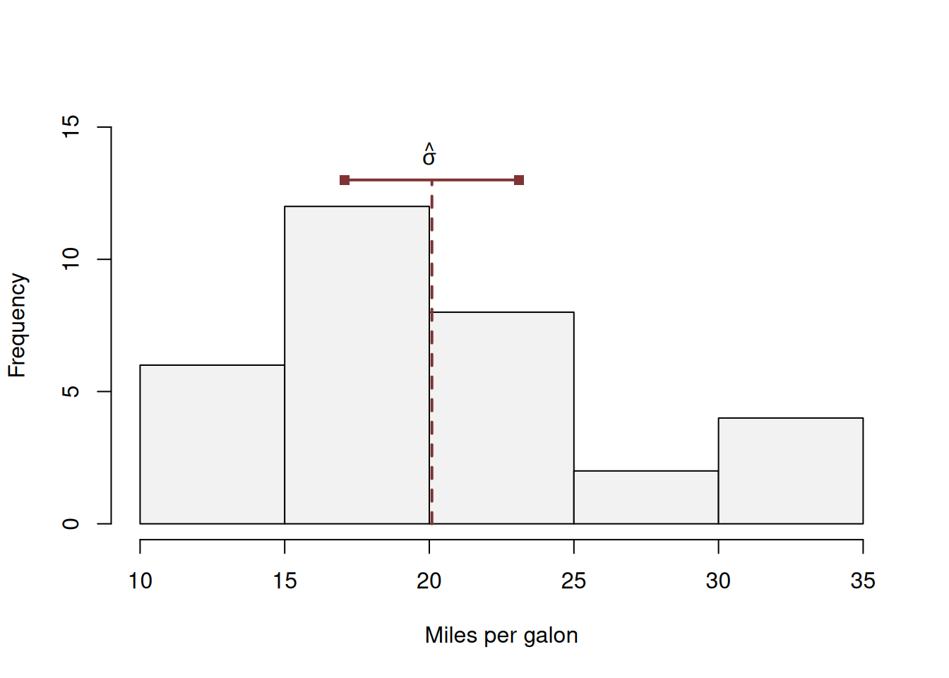
Figure 5.1: Visual presentation of standard deviation. The value of standard deviation corresponds to the segment between squares at the top of the histogram.
In Figure 5.1, we depict the distribution of the variable mpg using histogram (see Section 5.2) and show how the standard deviation relates to it – it is equal to the length of the segment above the histogram.
Coming back to the point about the asymmetry of the distribution of a variable in our example, we can investigate it further using skewness and kurtosis from timeDate package:
## [1] 0.610655
## attr(,"method")
## [1] "moment"## [1] -0.372766
## attr(,"method")
## [1] "excess"Skewness shows the asymmetry of distribution. If it is greater than zero, then the distribution has the long right tail. If it is equal to zero, then it is symmetric. It is calculated as: \[\begin{equation} \mathrm{skew}(y)= \frac{1}{n}\sum_{j=1}^n \frac{(y_j - \bar{y})^3}{\hat{\sigma}^3} . \tag{5.4} \end{equation}\]
Kurtosis shows the excess of distribution (fatness of tails) in comparison with the normal distribution. If it is equal to zero, then it is the same as for the normal distribution. Here how it is calculated: \[\begin{equation} \mathrm{kurt}(y)= \frac{1}{n}\sum_{j=1}^n \frac{(y_j - \bar{y})^4}{\hat{\sigma}^4} - 3 . \tag{5.5} \end{equation}\] Note that there is \(3\) in the formula. This is because the excess (which is the value without 3) of Normal distribution is equal to 3. Instead of dividing the value by 3 (which would make kurtosis easier to interpret), Karl Pearson has decided to use subtraction. The same formula (5.5) can be rewritten as: \[\begin{equation} \mathrm{kurt}(y)= \frac{1}{n}\sum_{j=1}^n \left(\frac{y_j - \bar{y}}{\hat{\sigma}}\right)^4 - 3 . \tag{5.6} \end{equation}\] Analysing the formula (5.6), we see that the impact of the deviations lying inside one \(\hat{\sigma}\) bounds are reduced, while those that lie outside, are increased. e.g. if the value \(y_j - \bar{y} > \hat{\sigma}\), then the value in the ratio will be greater than one (e.g. 2), thus increasing the final value (e.g. \(2^4=16\)), while in the opposite case of \(y_j - \bar{y} < \hat{\sigma}\), the ratio will be diminished (e.g. \(0.5^4 = 0.0625\)). After summing up all \(n\) values in (5.6), the values outside one \(\hat{\sigma}\) will have a bigger impact on the resulting kurtosis than those lying inside. So, kurtosis will be higher for the distributions with longer tails and in the cases when there are outliers in the data.
Based on all of this, we can conclude that the distribution of mpg is skewed and has the longer right tail. This is expected for such variable, because the cars that have higher mileage are not common in this dataset.
All the conventional statistics discussed above can be produced using the following summary for all variables in the dataset:
##       mpg             cyl             disp             hp
##  Min.   :10.40   Min.   :4.000   Min.   : 71.1   Min.   : 52.0
##  1st Qu.:15.43   1st Qu.:4.000   1st Qu.:120.8   1st Qu.: 96.5
##  Median :19.20   Median :6.000   Median :196.3   Median :123.0
##  Mean   :20.09   Mean   :6.188   Mean   :230.7   Mean   :146.7
##  3rd Qu.:22.80   3rd Qu.:8.000   3rd Qu.:326.0   3rd Qu.:180.0
##  Max.   :33.90   Max.   :8.000   Max.   :472.0   Max.   :335.0
##       drat             wt             qsec              vs             am
##  Min.   :2.760   Min.   :1.513   Min.   :14.50   V-shaped:18   automatic:19
##  1st Qu.:3.080   1st Qu.:2.581   1st Qu.:16.89   Straight:14   manual   :13
##  Median :3.695   Median :3.325   Median :17.71
##  Mean   :3.597   Mean   :3.217   Mean   :17.85
##  3rd Qu.:3.920   3rd Qu.:3.610   3rd Qu.:18.90
##  Max.   :4.930   Max.   :5.424   Max.   :22.90
##       gear            carb
##  Min.   :3.000   Min.   :1.000
##  1st Qu.:3.000   1st Qu.:2.000
##  Median :4.000   Median :2.000
##  Mean   :3.688   Mean   :2.812
##  3rd Qu.:4.000   3rd Qu.:4.000
##  Max.   :5.000   Max.   :8.000
Finally, one other moment that is often used in statistics is called “covariance”. It measures the joint variability of two variables and is calculated as: \[\begin{equation} \mathrm{cov}(x,y)= \frac{1}{n-1}\sum_{j=1}^n (x_j - \bar{x}) (y_j - \bar{y}) . \tag{5.7} \end{equation}\] Covariance is one of the more complicated moments to explain. It is equal to zero if one of the variables does not have any variability and otherwise can take any real value. We will discuss its meaning later in Section 10.2. One thing that we can note at this stage is that it is symmetric, meaning that the covariance between \(x\) and \(y\) is the same as the covariance between \(y\) and \(x\). This becomes apparent from the formula (5.7), where switching \(x_j\) with \(y_j\) and \(\bar{x}\) with \(\bar{y}\) will give you exactly the same formula.
Furthermore, the same formula can also be rewritten the following way, showing its connection with the variance and the expectations of random variables: \[\begin{equation} \mathrm{cov}(x,y)= \mathrm{E}(x \times y) - \mathrm{E}(x) \times \mathrm{E}(y). \tag{5.8} \end{equation}\] Comparing the formula (5.8) with (5.2), we can see that if \(x=y\) then the covariance transforms into the variance of the variable. So, you can think of a variance as a measure of a joint variability of a variable with itself.
Finally, if we have several random variables, we can create an object called “matrix” that would have variances of variables and covariances between them. This is sometimes convenient to do for some further analysis or for presenting the results. This is called “covariance matrix” or “variance-covariance matrix”. The idea is to group elements in a way that all variances lie on the diagonal, while the covariances would lie on the off-diagonals. In case of three variables (\(x\), \(y\) and \(z\)) it would look like this: \[\begin{equation} \begin{pmatrix} \mathrm{V}(x) & \mathrm{cov}(x,y) & \mathrm{cov}(x,z) \\ \mathrm{cov}(y,x) & \mathrm{V}(y) & \mathrm{cov}(y,z) \\ \mathrm{cov}(z,x) & \mathrm{cov}(z,y) & \mathrm{V}(z)\\ \end{pmatrix} \tag{5.9} \end{equation}\] Given the symmetry property of the covariance, the off-diagonal elements (such as \(\mathrm{cov}(x,y)\) and \(\mathrm{cov}(y,x)\)) would be the same.
We will come back to the covariance matrix in the future topics.