3.1 What is discrete distribution?
A random variable discussed in Section 2.2 can take a variety of values. For now we focus on discrete random variable, which means that it can take one of the several possible values with some probabilities. For example, if we roll two six-sided dices, we will have a variety of outcomes from 2 (both having score of one) to 12 (both having score of six), but not all outcomes will have equal probability. For example, there are different ways of obtaining score of 7: 1+6, 2+5, 3+4, 4+3, 5+2 and 6+1 - but there is only one way of obtaining 2: 1+1. In this case, we are dealing with a distribution of values from 2 to 12, where each value has its own probability of occurrence. This situation is shown in Figure 3.1.
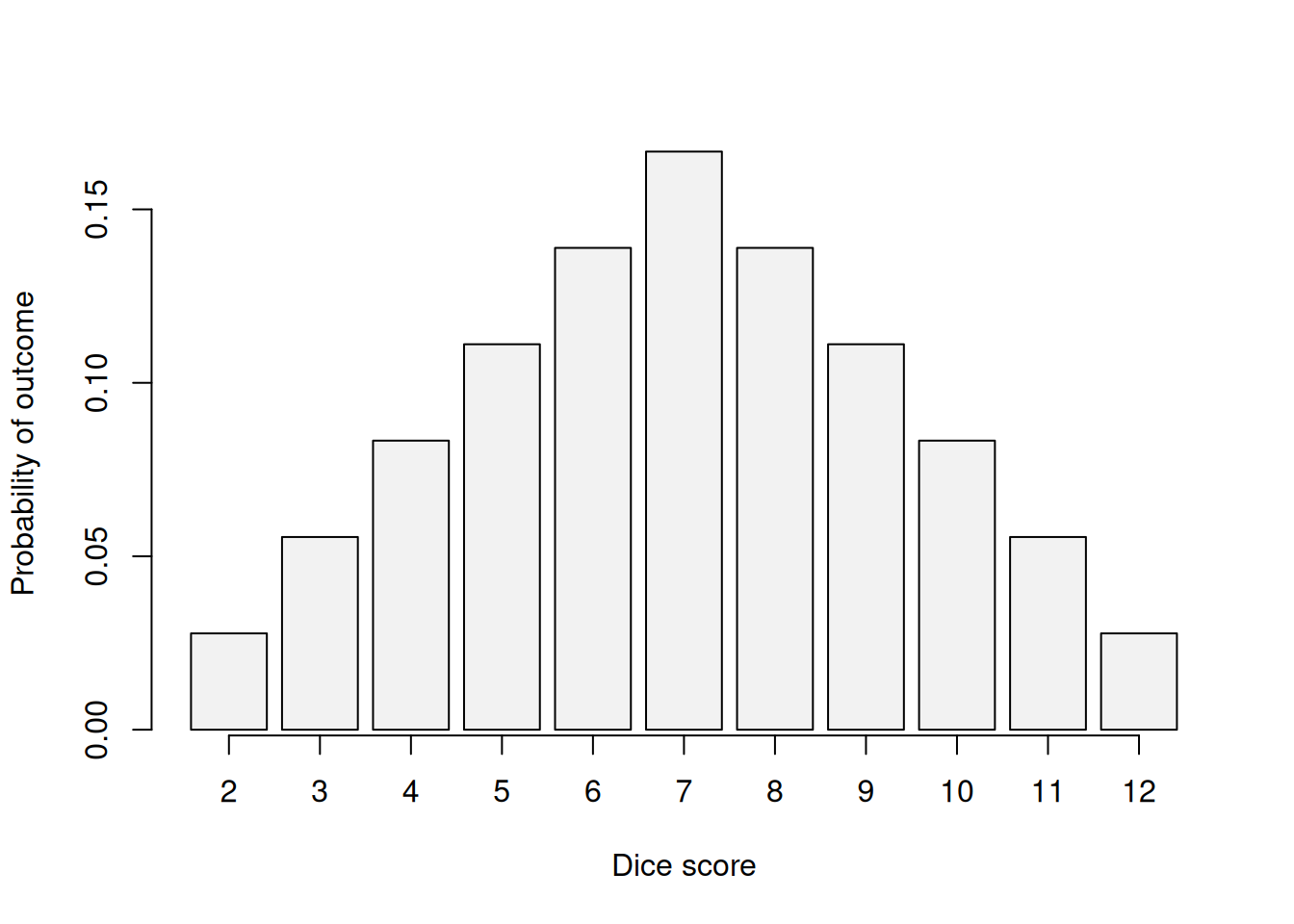
Figure 3.1: Distribution of outcomes for scores based on two dices.
As can be seen from Figure 3.1, the distribution of probabilities in this case is symmetric, the chances of having very low and very high scores are lower than the chance of having something closer to the middle. The probability of having 7 is the highest and is \(\frac{6}{36}=\frac{1}{6}\), which means that it will occur more often than other values if we repeat the experiment and roll the dices many times.
Any discrete distribution can be characterised using the following functions:
- Probability Mass Function (PMF);
- Cumulative Distribution Function (CDF);
- Moment Generation Function (MMF);
- Characteristic function (CF).
PMF is the function of probability of occurrence from specific values of random variable. An example of PMF is shown in Figure 3.1. Based on it, we can say what the probability of a specific outcome is for the random variable.
CDF shows the probability of the event lower than the specified one. For example, the probability of getting the score lower than 4 is \(\frac{1}{36}+\frac{2}{36}=\frac{1}{12}\), which corresponds to the sum of the first two bars in Figure 3.1. The CDF for our example is shown in Figure 3.2.
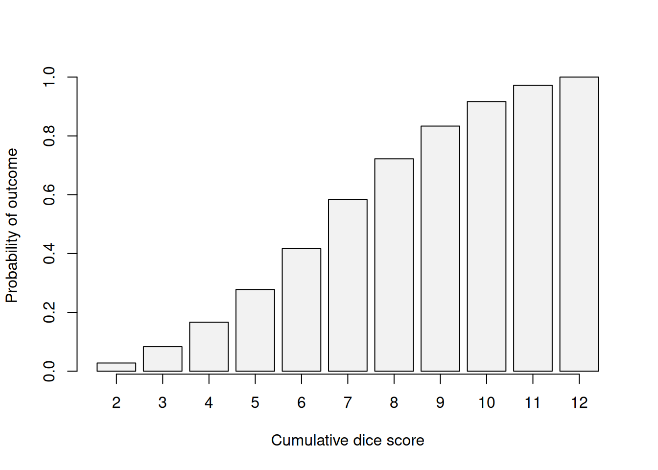
Figure 3.2: Cumulative distribution of outcomes for scores based on two dices.
Any CDF is equal to zero for the values below possible (e.g. it is impossible to get score of 1 rolling two dices) and is equal to one for the values at and above the maximum (if we roll two dices, the score will be below 13). Given that CDF shows probabilities, it can never be greater than one or lower than zero.
Finally, MGF and CF are the functions that allow obtaining the moments of distributions, such as mean, variance, skewness etc. We do not discuss these functions in detail in this textbook, and we will discuss the moments later in the Section 5.1.
Because we considered the discrete random variable, the distribution shown in Figure 3.1 is discrete as well.