3.4 Binomial distribution (Multiple coin tosses)
In the previous example with coin tossing we focused on the experiment that contained only one trial: toss a coin, see what score you got (zero or one). However, we could make the game more complicated and do it in, let us say, 10 trials. In this more complicated experiment we would sum up the scores to see what we get after those 10 trials. In theory, we can have any integer number from zero to ten, but the resulting score will be random and its chance of appearance will vary with the score. For example, we will get 0 only if in all 10 trials we get heads, while we can get 1 in a variety of ways:
- first trial is one and then the rest are zero;
- second trial is one and the rest are zero;
- etc.
This means that the score in this experiment will have a distribution of its own. But can we describe it somehow?
Yes, we can. The distribution that underlies this experiment is called “Binomial”. For the coin tossing experiment with 10 trials and \(p=0.5\) it looks like one shown in Figure 3.5.
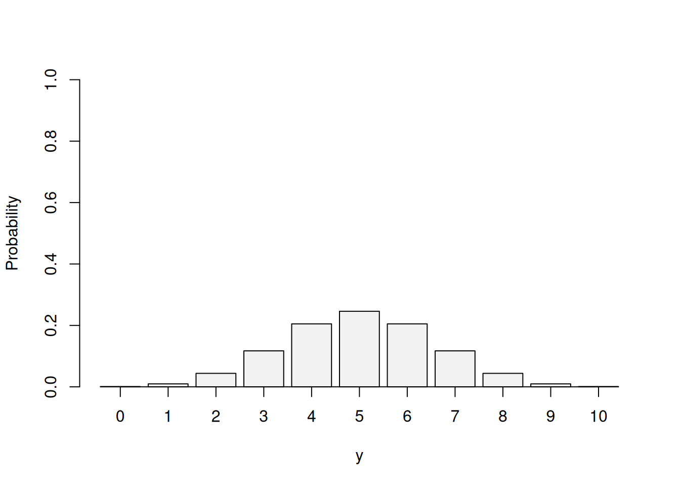
Figure 3.5: Probability Mass Function for Binomial distribution with p=0.5 and n=10.
From the Figure 3.5, we can see that the most probable outcome is the score of 5. This is because there are more ways of getting 5 than getting 4 in our example. In fact the number of ways can be calculated using Binomial coefficient, which is defined as: \[\begin{equation} \begin{pmatrix} n \\ k \end{pmatrix} = \frac{n!}{k!(n-k)!}, \tag{3.5} \end{equation}\] where \(k\) is the score of interest, \(n\) is the number of trials and \(!\) is the symbol for factorial. In our example, \(k=5\) and \(n=10\), meaning that we have: \[\begin{equation*} \begin{pmatrix} 10 \\ 5 \end{pmatrix} = \frac{10!}{5!(10-5)!} , \end{equation*}\] which can be calculated in R as:
and is equal to 252. Using this formula, we can calculate other scores for comparison:
##   0   1   2   3   4   5   6   7   8   9  10
##   1  10  45 120 210 252 210 120  45  10   1
Given that we throw the coin 10 times, there are overall \(2^{10}=1024\) theoretical of outcomes of this experiment, which allows calculating the probability of each outcome:
round((factorial(10) /
           (factorial(c(0:10))*factorial(10-c(0:10)))) /
          1024,3) |>
    setNames(nm=c(0:10))
## 0 1 2 3 4 5 6 7 8 9 10
## 0.001 0.010 0.044 0.117 0.205 0.246 0.205 0.117 0.044 0.010 0.001These probabilities can be obtained via the PMF of Binomial distribution:
\[\begin{equation}
f(k, n, p) = \begin{pmatrix} n \\ k \end{pmatrix} p^k (1-p)^{n-k} .
\tag{3.6}
\end{equation}\]
We will denote this distribution as \(\mathcal{Bi}(n, p)\). In R, this is implemented in the dbinom() function from stats package. Note that so far we assumed that \(p=0.5\), however in real life this is not necessarily the case.
Consider a problem of demand forecasting for expensive medical equipment in the UK. These are not typically bought in large quantities, and each hospital might need only one machine for their purposes, and that machine can last for many years. For demonstration purposes, assume that there is a fixed probability \(p=0.1\) that any given hospital decides to bye such machine. It is safe to assume that the probability that machine is needed in a hospital is independent of the probability in the other one. In this case, the distribution of demand for machines in the UK per year will be Binomial. For completeness of our example, assume that there are 20 hospitals in the country that might need such machine, then this will be characterised as \(\mathcal{Bi}(20, 0.1)\) and will be an asymmetric distribution, as shown in Figure 3.6.
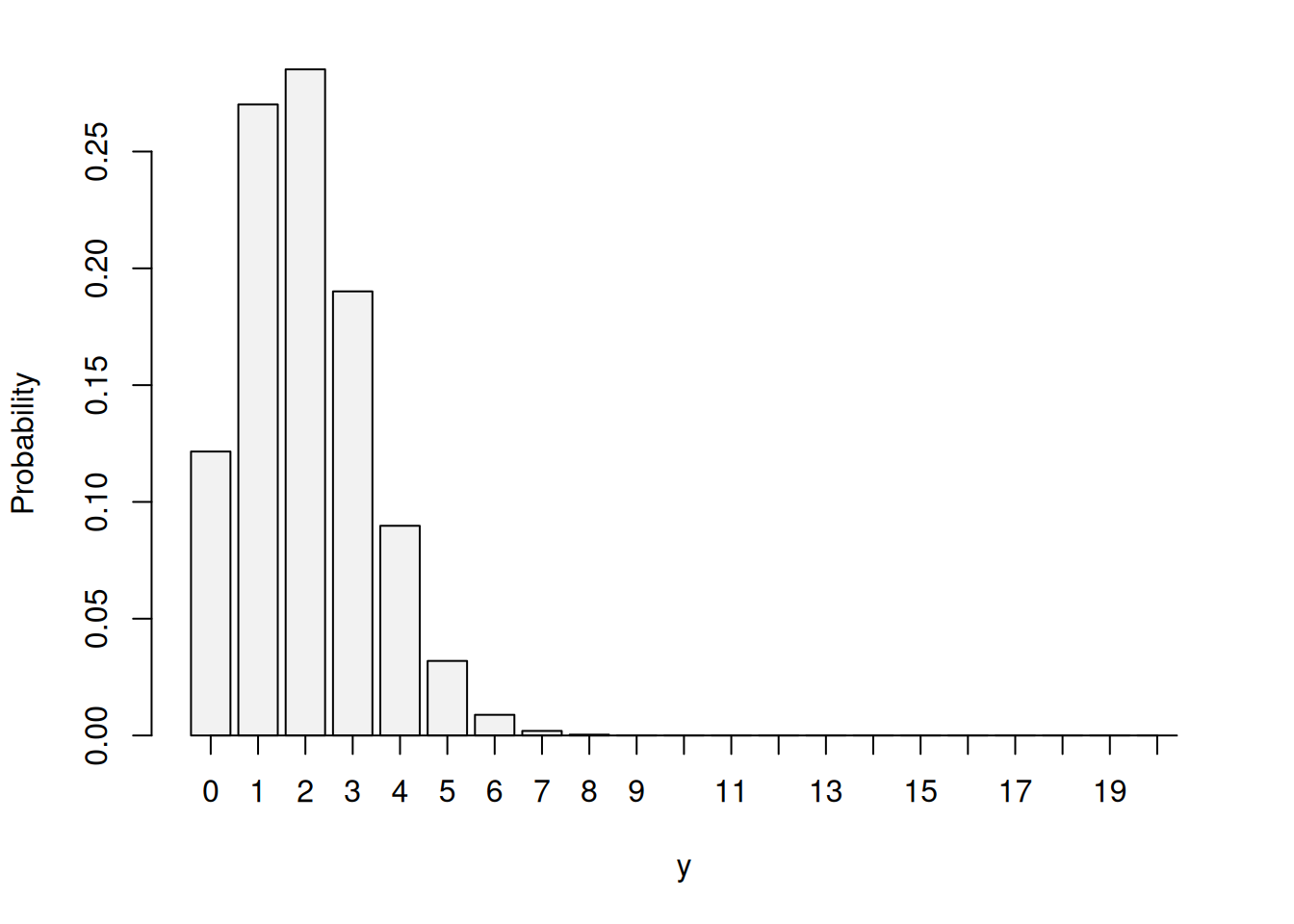
Figure 3.6: Probability Mass Function for Binomial distribution with p=0.1 and n=20.
From the Figure 3.6, it is clear that there is a high probability that only a few machines will be bought: 0, 1, 2 or 3. The probability that we will sell 10 is almost zero. We can also say that with the highest probability, the company will sell 2 machines. We could also use mean, saying how much the company will sell on average, which in Binomial distribution is calculated as \(n \times p\) and in our case is \(20 \times 0.1 = 2\). However, producing expensive medical equipment typically takes time and should be done in advance. So, if we told the company that they should produce only two, we might then face a situation, when the demand was higher (for example, 6) and they lost the sales.
So, while we already have a useful information about the distribution of demand in this situation, it is not helpful for decision making. What we could do is consider a case of satisfying, let us say, 99% of demand on machines. In our example, we should sum up the probabilities and find for which number of cases we get to 99%. Formally, this can be written as \(P(y<k)=0.99\) and we need to find \(k\). One way of doing this is by looking at cumulative distribution function of Binomial distribution, which is mathematically represented as: \[\begin{equation} F(k, n, p) = \sum_{i=0}^k \begin{pmatrix} n \\ i \end{pmatrix} p^i (1-p)^{n-i} . \tag{3.7} \end{equation}\]
This CDF in our example will have the shape shown in Figure 3.7.
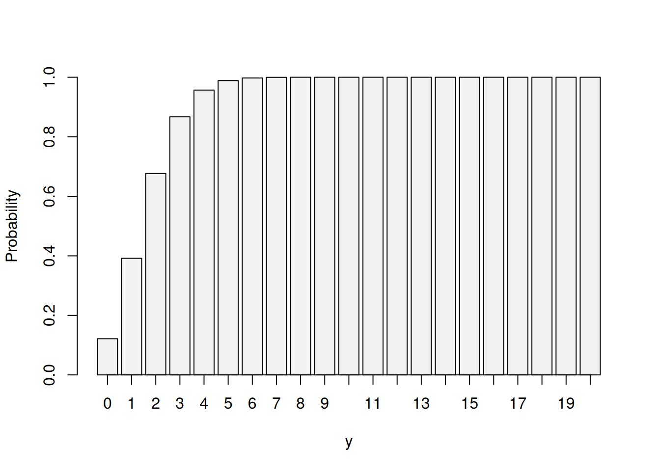
Figure 3.7: Cumulative Distribution Function for Binomial distribution with p=0.1 and n=20.
We can see from Figure 3.7 that the cumulative probability reaches value close to 1 after the outcome of 6. Numerically, for the \(y=6\), we have probability:
## [1] 0.9976139while for 5 we will have approximately 0.989. So, for our example, we should recommend the company to produce 6 machines - in this case in 99% of the cases the company will not loose the demand. Yes, in some cases, only 2 or 3 machines will be bought instead of 6, but at least the company will avoid a scenario, when their product is unavailable for clients.
We can get the same result by using Quantile Function, which is implemented in R as qbinom():
In some cases, we might need to know the mean and variance of the distribution. For the Binomial distribution, they can be calculated via the following formulae: \[\begin{equation} \mathrm{E}(y) = p \times n , \tag{3.8} \end{equation}\] and \[\begin{equation} \mathrm{V}(y) = p \times (1-p) \times n . \tag{3.9} \end{equation}\] So, in our situation the mean is \(20 \times 0.1 = 2\), while the variance is \(20 \times 0.1 \times 0.9 = 1.8\).
From the example above, we can take away several important characteristics ofthe Binomial distribution:
- There are many trials: we have many hospitals, each one of which can be considered as a ``trial’’;
- In each trial, there are only two outcomes: buy or do not buy;
- The probability of success (someone decides to buy the machine) is fixed between the trials: we assume that the probability that a hospital A decides to buy the machine is the same as for the hospital B;
- The trials are independent: if one hospital buys a machine, this should not impact the decision of another one;
- The number of trials \(n\) is fixed and known.
Final thing to note about the Binomial distribution is that with the growth of the number of trials it converges to the Normal one, no matter what the probability of success is. We can use this property to get answers about the Binomial distribution in those cases. We will discuss this in Section 4.3.
In R, the Binomial distribution is implemented via dbinom(), pbinom(), qbinom() and rbinom() from stats package. The functions have parameter size which is the number of trials \(n\), and parameter prob, which is a probability of success \(p\). If size=1, the distribution functions revert to the ones from Bernoulli distribution (Section 3.3).