Chapter 11 Multiple Linear Regression
Example 11.1 One of the problems that construction companies face is getting a good estimate of the budget needed to build something. Many companies tend to underestimate the costs and time the project will take. To address this, a mid-size company called “Eden city”, which specialises on construction of residential buildings, decided to take a more analytical approach to the problem. They have collected the data of their previous projects and needs help in building a model that would explain what forms the costs for different types of buildings. Their idea is to use this model during the business plan write-up phase to get an estimate of the future project, which they hope will be better than the ones they used before based on their pure judgment.
In this example, we are interested in the overall costs of construction (in thousands of pounds), which can be impacted by:
- The size of a building in squared meters,
- The cost of materials (in thousands of pounds),
- Type of building (detached, semi-detached, bungalow etc),
- How many projects the specific crew did before,
- Year when the project was started.
What else do you think can impact such costs in theory?
This data is available online:
Based on what we have discussed before, we can do analysis of measures of association and even build simple regression model (or several of them), but we acknowledge that in many real life situations, there are many factors that impact the variable of interest. In the example above, we have listed five explanatory variables that can be connected to the overall costs. This means that a basic bi-variate analysis (one variable vs the other) might not be sufficient. Furthermore, the relations between variables are typically complicated. So analysing, for example, only the relation between the cost of project and the size of building without considering the cost of materials might be misleading.
Here is how the bi-variate relations between the variables in our dataset look like (Figure 11.1):
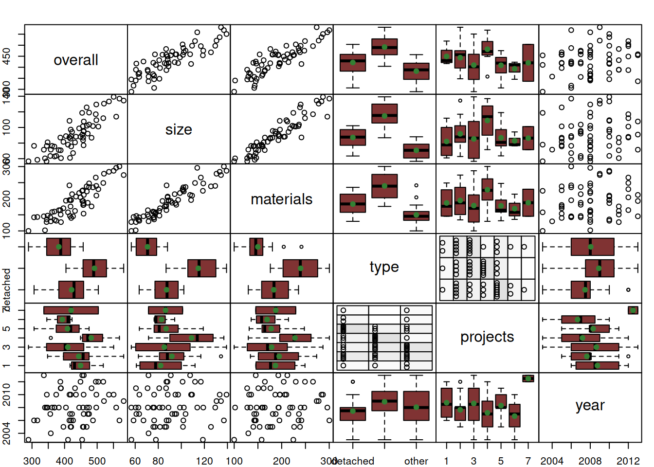
Figure 11.1: Spread plot between variables in the building costs dataset.
While the plot in Figure 11.1 gives a good idea about the relations, for example, between the size of property and the overall costs (it seems to be linear positive) or between material and the overall costs (linear positive again), it does not tell us much about the complex relation between one variable (overall costs) and several others.
All of this gives a motivation to having a so called “Multiple Linear Regression”, the model that expresses the relation between one variable and several of others. Mathematically, this is a straight forward extension of the simple linear regression model from Chapter 10, where we just add variables to the right-hand side of the equation. For example, if we had two variables impacting one (e.g. \(size\) of project and cost of \(materials\) vs \(overall\) cost of the project), we could write: \[\begin{equation} overall_j = \beta_0 + \beta_1 size_{j} + \beta_2 material_{j} + \epsilon_j , \tag{11.1} \end{equation}\] where \(beta_0\) is the intercept, and \(beta_1\), \(beta_2\) are the coefficients for the respective variables. The predicted overall costs can be calculated based on this model by dropping the error term \(\epsilon_j\): \[\begin{equation*} \widehat{overall}_j = \beta_0 + \beta_1 size_{j} + \beta_2 material_{j}. \end{equation*}\] While in the example with the Simple Linear Regression the predicted (or fitted) values implied drawing a line through the cloud of dots on the plane of the two variables, now we are talking about drawing a plane through the point in the three-dimensional space. It can be visualised in the following way (Figure 11.2):
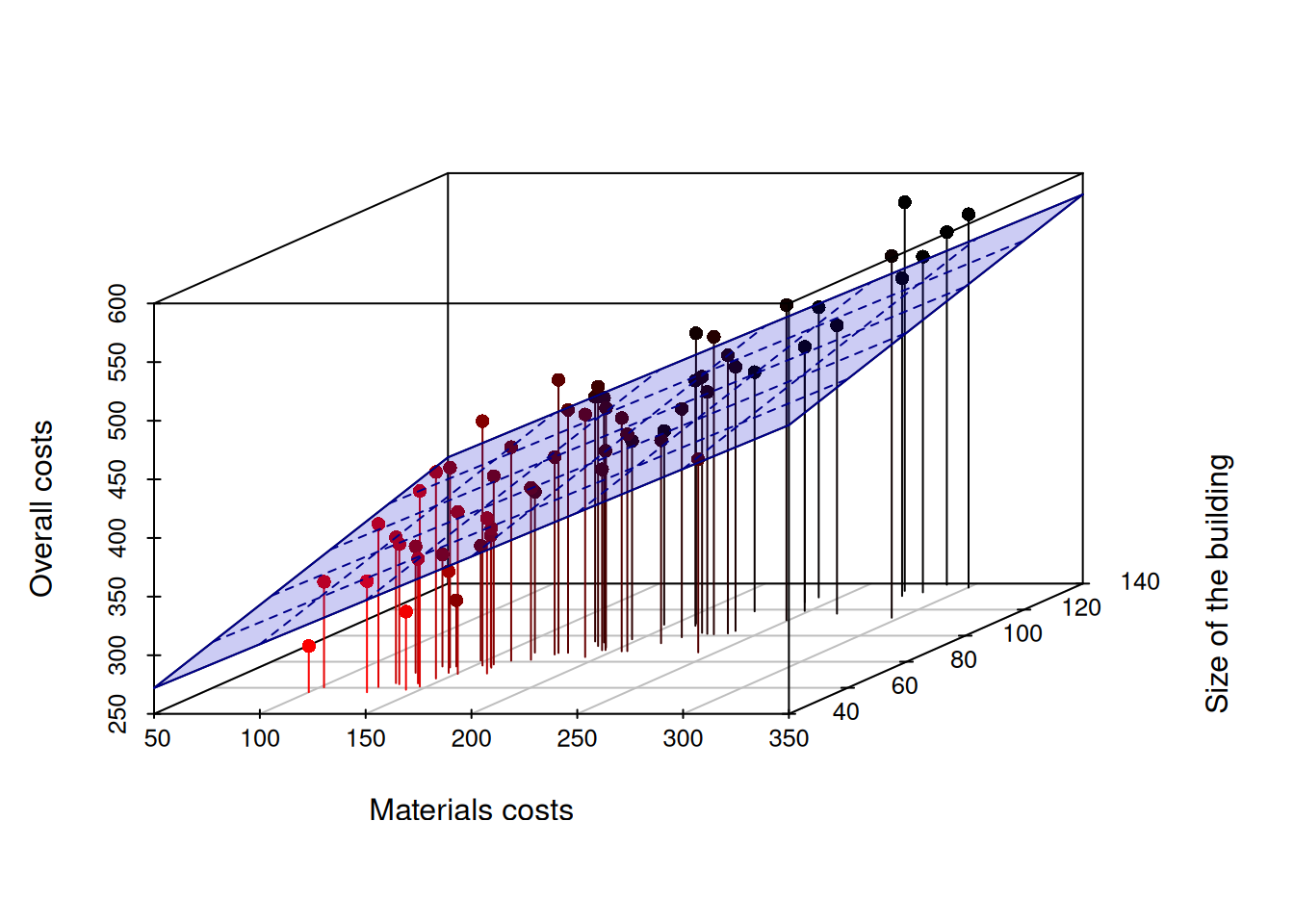
Figure 11.2: 3D scatterplot of Overall costs vs size of project and costs of materials.
The 3d image in Figure 11.2 is already hard to analyse, but at least it gives an idea of how the overall costs change with the change of materials costs and size of buildings. However, it would be impossible to produce a meaningful plot of overall costs from more than two variables. What the figure above gives us is the connection between the simple linear regression (which is just a straight line in the two-dimensional plane) and the multiple one (which is a plane in a multi-dimensional space).
In a more general way, the multiple linear regression can be written as: \[\begin{equation} y_j = \beta_0 + \beta_1 x_{1,j} + \beta_2 x_{2,j} + \dots + \beta_{k-1} x_{k-1,j} + \epsilon_j , \tag{11.2} \end{equation}\] where \(\beta_i\) is a \(i\)-th parameter for the respective \(i\)-th explanatory variable and there is \(k-1\) of them in the model, meaning that when we want to estimate this model, we will have \(k\) unknown parameters. The regression line of this model in population (aka expectation conditional on the values of explanatory variables) is: \[\begin{equation} \mu_{y,j} = \mathrm{E}(y_j | \mathbf{x}_j) = \beta_0 + \beta_1 x_{1,j} + \beta_2 x_{2,j} + \dots + \beta_{k-1} x_{k-1,j} . \tag{11.3} \end{equation}\] Furthermore, similar to how we discussed it in Chapter 10, when we want to estimate model (11.2), we should substitute all parameters \(\beta_j\) with their estimates \(b_j\): \[\begin{equation} \hat{y}_j = b_0 + b_1 x_{1,j} + b_2 x_{2,j} + \dots + b_{k-1} x_{k-1,j} . \tag{11.4} \end{equation}\] Similar to the Simple Linear Regression, each parameter in equation (11.4) represents the slope for the respective variable, showing how on average the value of the response variable (overall costs in our example) changes with the change of each variable.
11.0.1 A couple of notes about the “true” model
One thing we should discuss briefly is the term “true” model, which was mentioned in Subsection 1.1.1. The whole idea of the true model implies that this is a model that has the following important properties:
- It is applied to the population of data (i.e. all the data in the universe);
- It has all the important variables in it, i.e. there are no omitted variables that could impact the response variable;
- All included important variables are in the correct format. i.e., all necessary transformations are done;
- Because of (1) - (3), the error term of the model does not have any structure left, and represents small random fluctuations around the structure that cannot be captured by any other variables;
- Because of (4), the error term has a zero expectation;
- As a result of (4), the error term cannot be correlated with any of the variables, either included in the model or omitted by it. Having this the other way around would imply that there is some structure left in the error, which should be transferred away from it;
- Similarly, the error term cannot be related to its values on other observations. This issue can potentially appear on time series, where an error of an applied model on Monday can be related to the error on Tuesday. But when we talk about the true model, the errors cannot be related, otherwise this would imply that we missed some structure, thus violating (1) - (3);
- In the simple case of a linear model that we are discussing in this Chapter, the error term also has some fixed variance;
- The parameters of the model should also be independent of the error term for the same reason (4).
In the simple case of a linear true model, it can be represented as: \[\begin{equation} y_j = \mu_{y,j} + \epsilon_j . \tag{1.1} \end{equation}\] where \(\mu_j\) is the structure that we can capture in theory with the correct set of explanatory variables, and \(\epsilon_j\) is the true error term that mathematically has \(\mathrm{E}(\epsilon_j)=0\) due to (5) and \(\mathrm{V}(\epsilon_j)=\sigma^2\) due to (8). The property (6) can be written mathematically as \(\mathrm{E}(x_{i,j}\epsilon_j)=0\) for any \(i\) and \(j\). This model can be called “linear” or “additive”, because the structure and the error interact are added in one linear equation. But the true model can be more complicated and might contain non-linear structure or some complicated interactions between variables and the error term.
For now, we focus on the model (1.1) and we assume that when we estimate a model, we know its form and have all the necessary variables. We will discuss what happens when this is violated in Chapter 15.