2.4 Multiplication of probabilities: Calculating “AND” Probability
Consider an example: Jane has a 0.7 probability of writing a page of coursework with no spelling mistakes. This means she has a 0.3 probability of making at least one mistake on a given page. She is writing a 3-page assignment, and what happens on the first page in no way affects what happens on the other pages. What is the probability that she will have no spelling mistakes on at least one of the three pages?
To answer this question, we need to use the Multiplication Law. In this specific example, we can use the simplified version of it because the events (a mistake on a page) are independent (as stated in the setting above).
Definition 2.2 Independent events are the events where the occurrence of one has no influence on the probability of the other.
2.4.1 Independent Events
Calculating the probability of “at least one” success implies that Jane made no mistakes in one of these situations:
- No mistakes on all three pages;
- Mistake on exactly one page: either the first, the second, or the third;
- Mistakes on exactly two pages: either first and second, or first and third, or second and third.
Calculating all probabilities and summing them up is cumbersome. Luckily, there is a simpler way of getting the answer: to use the complement rule, which states that the probability of an event happening is 1 minus the probability of it not happening. In our case, the “not happening” means that Jane will have spelling mistakes on every page (this is the only other option left). Mathematically it can be written down as:
\[\begin{equation*} P(\text{No mistakes on at least one page}) = 1 - P(\text{Mistakes on all pages}) \end{equation*}\]
To calculate the probability of the complementary event (mistakes on all 3 pages), we can use the Multiplication Law. Given that the events are independent, all we need to do is multiply the probability of having a mistake on the first page by the probability of having a mistake on the second and then the probability of having a mistake on the third page:
\[\begin{equation*} P(\text{Mistakes on all pages}) = P(M_1 \cap M_2 \cap M_3) = P(M_1) × P(M_2) × P(M_3) = 0.3 × 0.3 × 0.3 = 0.3^3 = 0.027. \end{equation*}\]
After that, we can the complement rule to answer the original question:
\[\begin{equation*} P(\text{No mistakes on at least one page}) = 1 - P(\text{Mistakes on all pages}) = 1 -0.027 = 0.973 \end{equation*}\]
So, there is a 97.3% chance that at least one page will be free of spelling mistakes. This example illustrates the Multiplication Law for Independent Events, which can be written mathematically as: \[\begin{equation} P(A \cap B) = P(A) \times P(B) . \tag{2.5} \end{equation}\]
Visually, we could draw a Venn diagram to understand what specific area we are talking about when we use the multiplication law (Figure 2.3).
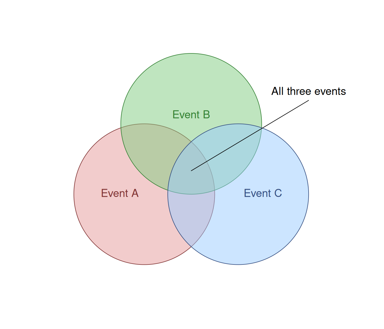
Figure 2.3: Venn diagram for three events.
In that diagram, the multiplication corresponds to the area in the intersection of circles. If the events are independent, the outcome “every page contains a mistake” corresponds to the area for “all three events”, i.e. \(P(A \cap B \cap C) = P(A) \times P(B) \times P(C)\), as we saw in the example above.
2.4.2 Dependent Events and Conditional Probability
The situation changes when we deal with dependent events, where the outcome of the first event impacts the probability of the second.
Consider another example: in a class of 6 students, 4 are secretly vampires. The teacher randomly chooses 2 students. What is the probability that neither of the two chosen students are vampires?
These events are dependent because as soon as the teacher chooses one student, the sample size changes and the probabilities for the rest would change. This is called “sampling without replacement”. The selection of the first student changes the composition of the group from which the second student is chosen. To handle this, we must use Conditional Probability.
To better understand the situation, we can draw a tree diagram, which depicts the possible situations (Figure 2.4).
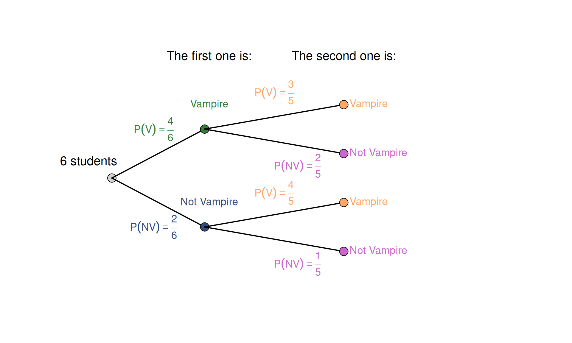
Figure 2.4: Tree diagram for the vampire example.
In this diagram, when we pick the first student, we reduce the pool of the students to choose from from 6 to 5. This also changes the probabilities for students being and not being vampires, depending on whom we picked in the first step. The probabilities on the second step now become conditional on the choice made in the first step and are denoted in general as \(P(A|B)\), which can be read as “probability of the outcome A, given the outcome B”. In our terms, we can denote, for example, the probability that the student is not a vampire, given that the first one was not a vampire, as \(P(NV_2 | NV_1)\).
Using the Multiplication law, we need to take the probability of a student being not a vampire in the first step and multiply it by the probability of the student not being a vampire in the second step, given that the first one was not a vampire. Mathematically, it can be written:
\[\begin{equation*} P(NV_1) \times P(NV_2 | NV_1) = \frac{2}{6} \times \frac{1}{5} = \frac{2}{30} = \frac{1}{15} \approx 0.067. \end{equation*}\]
So the probability of picking two non-vampire students in our example is only 6.7%.
2.4.3 General Multiplication Law
The Multiplication Law is used to determine the probability of two or more events occurring in sequence or simultaneously - an ‘AND’ scenario. In business, success often depends on a chain of events, where every link must hold. The Multiplication Law is the tool we can use to quantify the probability of that entire chain succeeding, whether in quality control, financial modelling, or project management. Mathematically, we use the notation \(P(B|A)\) to represent “the probability of event B occurring, given that event A has already occurred”.
The dependent events example leads us to the formal statement of the general rule.
The General Multiplication Law for Probabilities is written mathematically as: \[\begin{equation} P(A \cap B) = P(B) \times P(A|B) . \tag{2.6} \end{equation}\] In case of the independence, the conditional probability becomes just an unconditional one: \(P(A|B)=P(A)\).
By algebraically rearranging formula (2.6), we arrive at the formal definition of Conditional Probability: \[\begin{equation} P(A|B) = \frac{P(A \cap B)} {P(B)}. \tag{2.7} \end{equation}\]
This rearrangement is more than just algebra; it provides the fundamental definition of conditional probability. It defines the probability of “A given B” as the proportion of B outcomes that also include A. Visually, this can be shown in Figure 2.5. There, the conditional probability of A given B would correspond to the proportion of the areas \(A \cap B\) (intersection of events) to the overall area of B.
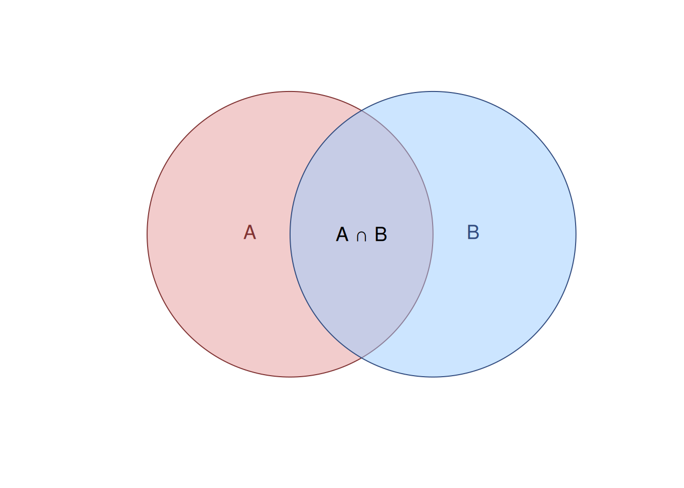
Figure 2.5: Venn diagram for the conditional probability explanation.