6.4 Properties of estimators
Before we move further, we need to agree what the term “estimator” means, which will be used several times further in this textbook:
- Estimate of a parameter is a result of application of a statistical procedure to the sample of data for obtaining some coefficients of a model. The value that we get when using the arithmetic mean on a sample of data is an estimate of the population mean;
- Estimator is the rule for calculating estimates of parameters based on a sample of data. For example, arithmetic mean itself is an estimator of the population mean. Another example would be method of Ordinary Least Squares, which is a rule for producing estimates of parameters of a regression model and thus an estimator.
In this section, we discuss such terms as bias, efficiency and consistency of estimates of parameters, which are directly related to LLN and CLT. Although there are strict statistical definitions of the aforementioned terms (you can easily find them in Wikipedia or anywhere else), we want to discuss them only in a general way, explaining the ideas behind them.
Note that all the discussions in this chapter relate to the estimates of parameters, not to the distribution of a random variable itself. A common mistake that students make when studying statistics, is that they think that the properties apply to the variable \(y_j\) instead of the estimate of its parameters (e.g. mean of \(y_j\)).
6.4.1 Bias
Bias refers to the expected difference between the estimated value of parameter (on a specific sample) and the “true” one (in the true model). Having unbiased estimates of parameters is important because they should lead to more accurate forecasts (at least in theory). For example, if the estimated parameter is equal to zero, while in fact it should be 0.5, then the model would not take the provided information into account correctly and as a result will produce less accurate point forecasts and incorrect prediction intervals. In inventory context this may mean that we constantly order 100 units less than needed only because the parameter is lower than it should be.
The classical example of bias in statistics is the estimation of variance in sample. The following formula gives biased estimate of variance in sample: \[\begin{equation} \mathrm{V}(y) = \frac{1}{n} \sum_{j=1}^n \left( y_j - \bar{y} \right)^2, \tag{6.1} \end{equation}\] where \(n\) is the sample size and \(\bar{y} = \frac{1}{n} \sum_{j=1}^n y_j\) is the mean of the data. There is a lot of proofs in the literature of this issue (even Wikipedia (2020a) has one), we will not spend time on that. Instead, we will see this effect in the following simple simulation experiment:
mu <- 100
sigma <- 10
nIterations <- 1000
# Generate data from normal distribution, 10,000 observations
y <- rnorm(10000,mu,sigma)
# This is the function, which will calculate the two variances
varFunction <- function(y){
   return(c(var(y), mean((y-mean(y))^2)))
}
# Calculate biased and unbiased variances for the sample of 30 observations,
# repeat nIterations times
varValues <- replicate(nIterations, varFunction(sample(y,30)))
This way we have generated 1000 samples with 30 observations and calculated variances using the formulae (6.1) and the corrected one for each step. Now we can plot it in order to see how it worked out:
par(mfcol=c(1,2))
# Histogram of the biased estimate
hist(varValues[2,], xlab="V(y)", ylab="y", main="Biased estimate of V(y)",
     col=17)
abline(v=mean(varValues[2,]), col=2, lwd=2)
legend("topright",legend=TeX(paste0("E$\\left(V(y)\\right)$=",round(mean(varValues[2,]),2))),
       lwd=2, col=2)

# Histogram of unbiased estimate
hist(varValues[1,], xlab="V(y)", ylab="y", main="Unbiased estimate of V(y)",
     col=17)
abline(v=mean(varValues[1,]), col=2, lwd=2)
legend("topright",legend=TeX(paste0("E$\\left(V(y)\\right)$=",round(mean(varValues[1,]),2))),
       lwd=2, col=2)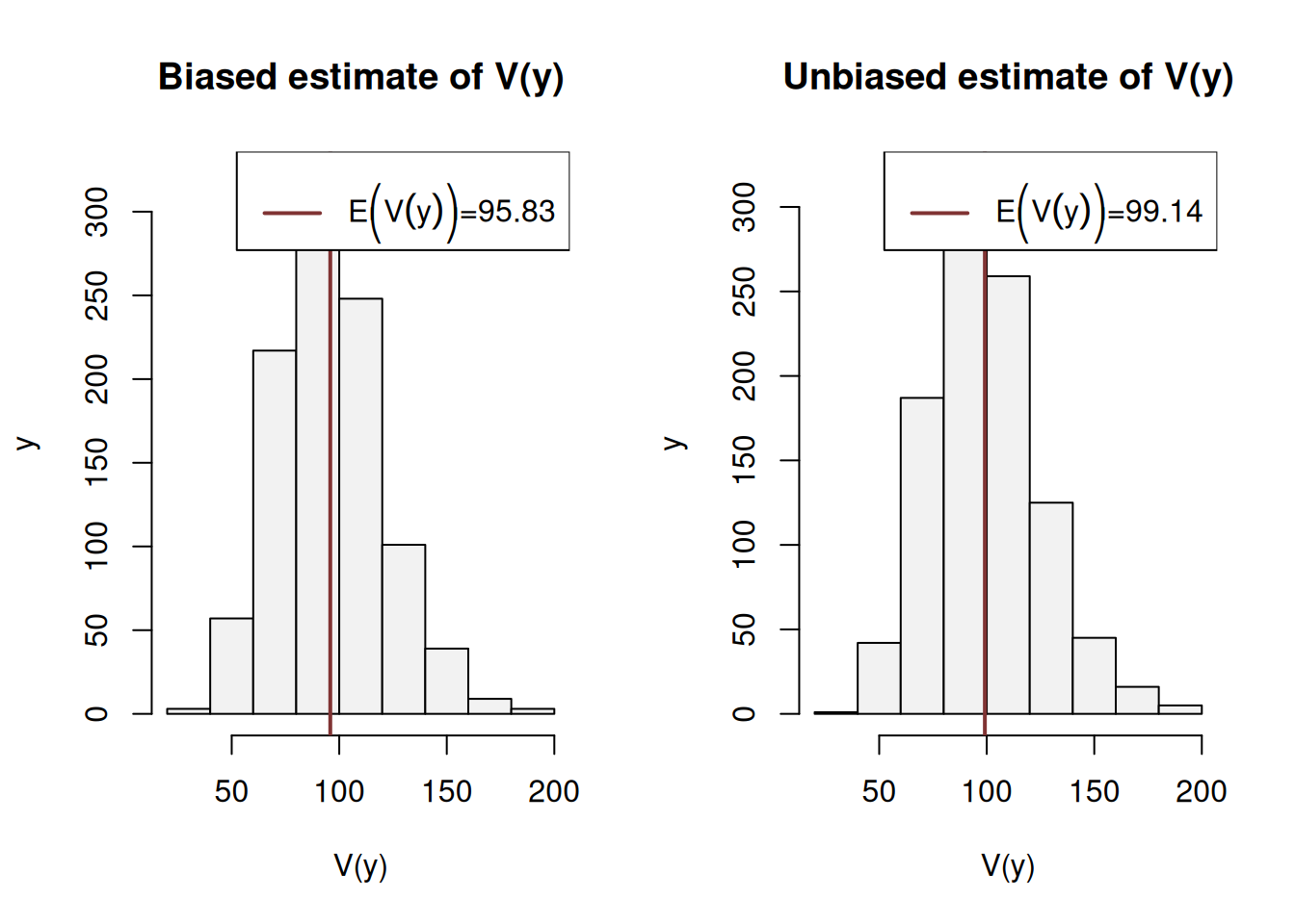
Figure 6.11: Histograms for biased and unbiased estimates of variance.
Every run of this experiment will produce different plots, but typically what we will see is that, the biased estimate of variance (the histogram on the right hand side of the plot) will have lower mean than the unbiased one. This is the graphical example of the effect of not taking the number of estimated parameters into account. The correct formula for the unbiased estimate of variance is: \[\begin{equation} s^2 = \frac{1}{n-k} \sum_{j=1}^n \left( y_j - \bar{y} \right)^2, \tag{6.2} \end{equation}\] where \(k\) is the number of all independent estimated parameters. In this simple example \(k=1\), because we only estimate mean (the variance is based on it). Analysing the formulae (6.1) and (6.2), we can say that with the increase of the sample size, the bias will disappear and the two formulae will give almost the same results: when the sample size \(n\) becomes big enough, the difference between the two becomes negligible. This is the graphical presentation of the bias in the estimator.
6.4.2 Efficiency
Efficiency means, if the sample size increases, then the estimated parameters will not change substantially, they will vary in a narrow range (variance of estimates will be small). In the case with inefficient estimates the increase of sample size from 50 to 51 observations may lead to the change of a parameter from 0.1 to, let’s say, 10. This is bad because the values of parameters usually influence both point forecasts and prediction intervals. As a result the inventory decision may differ radically from day to day. For example, we may decide that we urgently need 1000 units of product on Monday, and order it just to realise on Tuesday that we only need 100. Obviously this is an exaggeration, but no one wants to deal with such an erratically behaving model, so we need to have efficient estimates of parameters.
Another classical example of not efficient estimator is the median, when used on the data that follows Normal distribution. Here is a simple experiment demonstrating the idea:
set.seed(42)
mu <- 100
sigma <- 10
nIterations <- 500
obs <- 100
varMeanValues <- vector("numeric",obs)
varMedianValues <- vector("numeric",obs)
y <- rnorm(100000,mu,sigma)
for(i in 1:obs){
    ySample <- replicate(nIterations,sample(y,i*100))
    varMeanValues[i] <- var(apply(ySample,2,mean))
    varMedianValues[i] <- var(apply(ySample,2,median))
}
In order to establish the efficiency of the estimators, we will take their variances and look at the ratio of mean over median. If both are equally efficient, then this ratio will be equal to one. If the mean is more efficient than the median, then the ratio will be less than one:
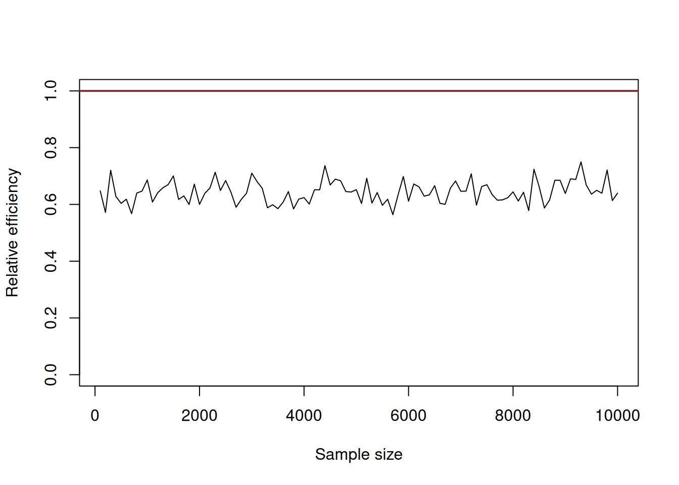
Figure 6.12: An example of a relatively inefficient estimator.
What we should typically see on this graph, is that the black line should be below the red one, indicating that the variance of mean is lower than the variance of the median. This means that mean is more efficient estimator of the true location of the distribution \(\mu\) than the median. In fact, it is easy to proove that asymptotically the mean will be 1.57 times more efficient than median (Wikipedia, 2020b) (so, the line should converge approximately to the value of 0.64).
6.4.3 Consistency
Consistency means that our estimates of parameters will get closer to the stable values (true value in the population) with the increase of the sample size. This follows directly from LLN and is important because in the opposite case estimates of parameters will diverge and become less and less realistic. This once again influences both point forecasts and prediction intervals, which will be less meaningful than they should have been. In a way consistency means that with the increase of the sample size the parameters will become more efficient and less biased. This in turn means that the more observations we have, the better.
An example of inconsistent estimator is Chebyshev (or max norm) metric. It is formulated the following way: \[\begin{equation} \mathrm{LMax} = \max \left(|y_1-\hat{y}|, |y_2-\hat{y}|, \dots, |y_n-\hat{y}| \right). \tag{6.3} \end{equation}\] Minimising this norm, we can get an estimate \(\hat{y}\) of the location parameter \(\mu\). The simulation experiment becomes a bit more tricky in this situation, but here is the code to generate the estimates of the location parameter:
# L-max loss function
LMax <- function(y){
    estimator <- function(par){
        return(max(abs(y-par)));
    }

    return(optim(mean(y), fn=estimator, method="Brent",
                 lower=min(y), upper=max(y)));
}

set.seed(43)
mu <- 100
sigma <- 10
nIterations <- 1000
y <- rnorm(10000, mu, sigma)
LMaxEstimates <- vector("numeric", nIterations)
for(i in 1:nIterations){
    LMaxEstimates[i] <- LMax(y[1:(i*10)])$par;
}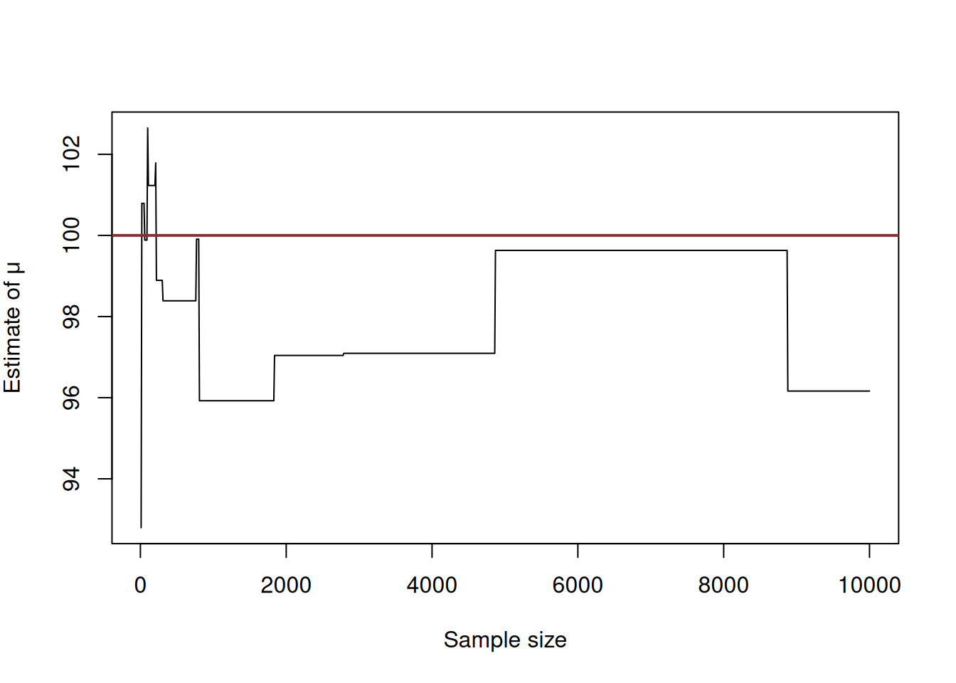
Figure 6.13: An example of inconsistent estimator.
While in the example with bias we could see that the lines converge to the red line (the true value) with the increase of the sample size, the Chebyshev metric example shows that the line does not approach the true one, even when the sample size is 10000 observations. The conclusion is that when Chebyshev metric is used, it produces inconsistent estimates of parameters.
Remark. There is a prejudice in the world of practitioners that the situation in the market changes so fast that the old observations become useless very fast. As a result many companies just throw away the old data. Although, in general the statement about the market changes is true, the forecasters tend to work with the models that take this into account (e.g. Exponential smoothing, ARIMA, discussed in this book). These models adapt to the potential changes. So, we may benefit from the old data because it allows us getting more consistent estimates of parameters. Just keep in mind, that you can always remove the annoying bits of data but you can never un-throw away the data.
6.4.4 Asymptotic normality
Finally, asymptotic normality is not critical, but in many cases is a desired, useful property of estimates. What it tells us is that the distribution of the estimate of parameter will be well behaved with a specific mean (typically equal to \(\mu\)) and a fixed variance. This follows directly from CLT. Some of the statistical tests and mathematical derivations rely on this assumption. For example, when one conducts a significance test for parameters of model, this assumption is implied in the process. If the distribution is not Normal, then the confidence intervals constructed for the parameters will be wrong together with the respective t- and p- values.
Another important aspect to cover is what the term asymptotic, which we have already used, means in our context. Here and after in this book, when this word is used, we refer to an unrealistic hypothetical situation of having all the data in the multiverse, where the time index \(t \rightarrow \infty\). While this is impossible in practice, the idea is useful, because asymptotic behaviour of estimators and models is helpful on large samples of data. Besides, even if we deal with small samples, it is good to know what to expect to happen if the sample size increases.
6.4.5 Why having biased estimate can be better than having the inefficient one?
It might not be clear to everyone why the model with some bias in it might be better than the model with high variance. In order to answer this question, consider the situation, where we want to estimate the value of parameter \(\mu\), and we have two methods to do that. Given that we work on a sample of data, the estimates will have some sorts of distributions, shown in Figure 6.14.
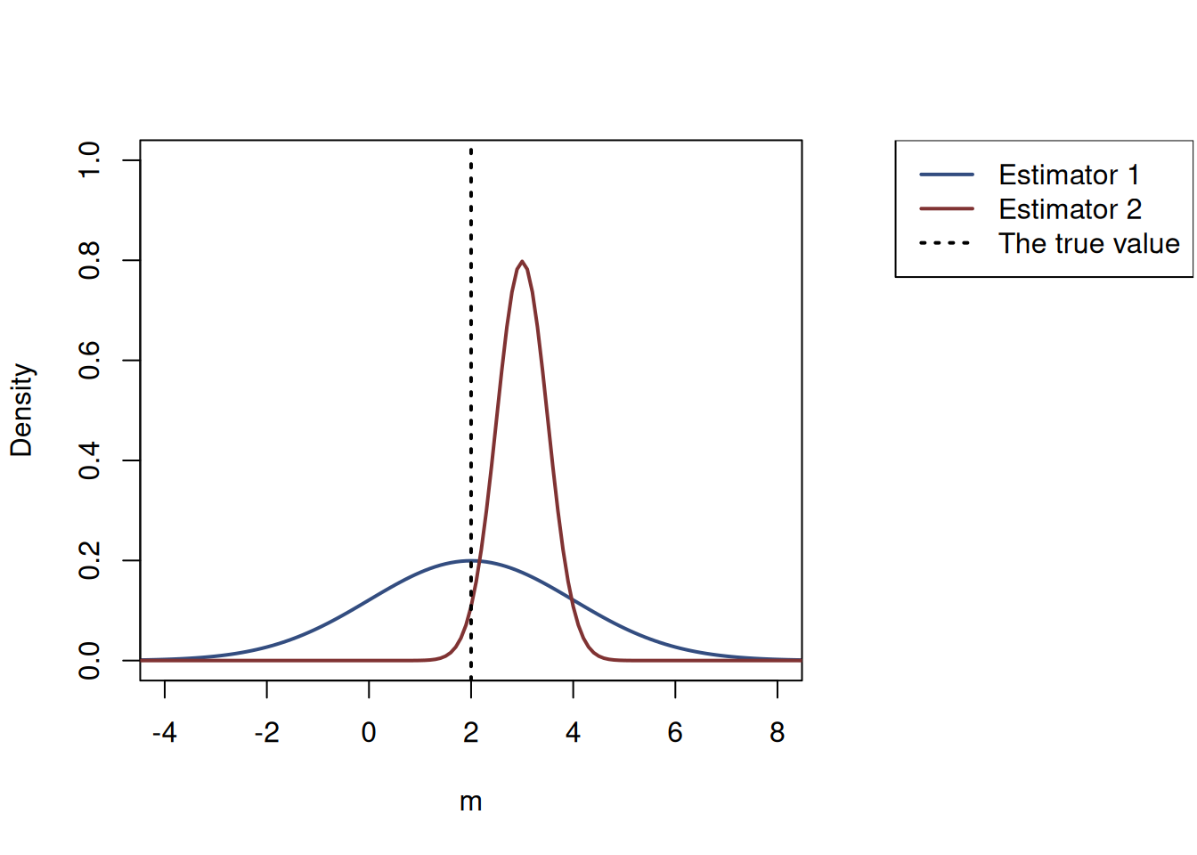
Figure 6.14: Example of two estimators of a parameter.
Which of the two estimators would you prefer: the first one or the second one? The conventional statistician might choose Estimator 1, because it produces the unbiased estimates of parameter, meaning that on average we will have the correct value of the true parameter. However, if we rephrase the question slightly, making it more realistic, the answer would probably change: “Which of the two estimators would you prefer on small sample?”. In this situation, we understand that we have limited data and need to make a decision based on what we have on hands, we might not be able to rely on asymptotic properties, on LLN and CLT (Chapter 6). If we choose Estimator 1, then on our specific sample, we might end up easily with a value for \(m\) of -2, 0 or 6, just due to the pure chance - this is how wide the distribution is. On the other hand, if we choose the Estimator 2, we will end up with the value, which will be close to the true one: 2.5, 3 or 4. Yes, this value will be typically higher than needed, but at least it will not lead us to confusing conclusions on the data we have. Having said that, if the bias was too high (e.g. if the distribution of the Estimator 2 was placed around -4), the estimator might become unreliable, so there should be some balance in how much bias one should impose.
Example 6.1 In a computer game Diablo II (by Blizzard North), there are two spells, which might be considered as similar in terms of damage to monsters: Lightning and Glacial Spike. On the first level, the Lightning does random damage from 1 to 43, while the Glacial Spike does randomly 17 to 26. Assuming that the distributions of damage are uniform in both cases, we would conclude that on average the Lightning does slightly more damage than the Glacial Spike: \(\frac{1}{2}(43+1)=22\) vs \(\frac{1}{2}(17+26)=21.5\). However, the Lightning has much higher variability, and is less efficient in killing monsters than the Glacial Spike: it has variance of \(\frac{1}{12}(43-1)^2 = 147\) versus \(\frac{1}{12}(26-17)^2 = 6.75\) of the Glacial Spike. This means that each time a player shoots the Lightning, there is a chance that it will do less damage than the Glacial Spike (for example, in \(\frac{(17-1)}{(43-1)} \approx 38\)% of the cases Lightning will do less damage than the lowest possible damage of the Glacial Spike). This means that if one needs to choose, which of the spells to use in a battle, the Glacial Spike would be a safer option, as each specific shot will not be as weak as it could be in the case of the Lightning. But if a player casts both spells many times, then asymptotically the Lightning will be better than Glacial Spike, as it would do more damage on average.