4.4 Log-Normal distribution
Log-Normal distribution is closely related to the Normal one and is supported for the positive values of \(y\). It is defined as a distribution arising after a transformation of a variable \(x=\log(y)\) or equivalently \(y=e^x\). It is said that \(y=e^x \sim \log\mathcal{N}(\mu_y, \sigma^2)\) if \(\log y = x \sim \mathcal{N}(\mu_y, \sigma^2)\). Figure 4.15 shows the connection between Normal and Log-Normal distributions. In that plot, we can see how the density changes because of the \(y=e^x\) transformation.
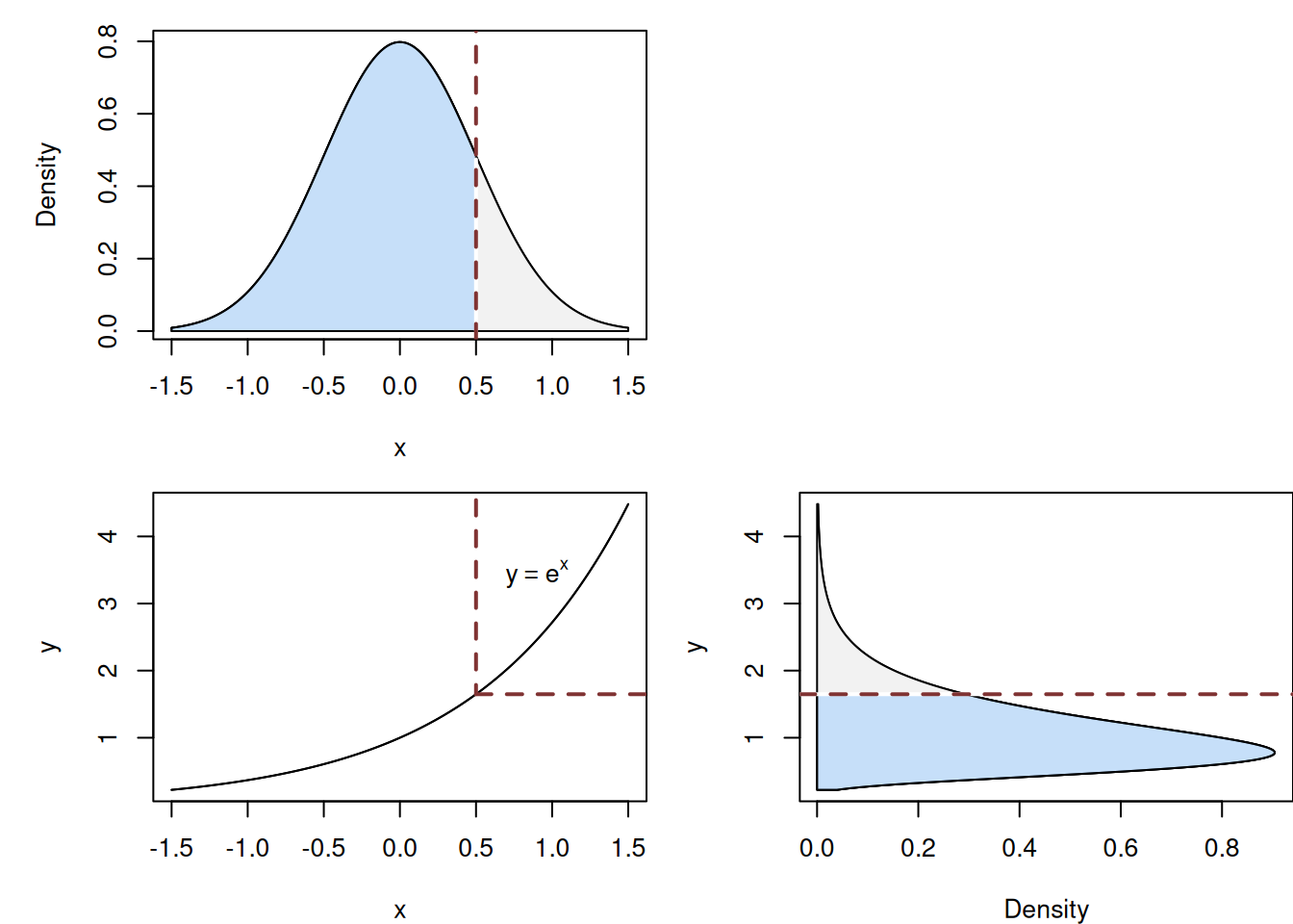
Figure 4.15: Connection between Normal and Log-Normal distributions
The dark areas on the plots in Figure 4.15 show equal probabilities for the Normal and the Log-Normal distributions obtained via specific quantiles. This demonstrates that in order to obtain a quantile of the Log-Normal distribution for \(y\), we need to produce a quantile from the Normal one for \(x\) and then exponentiate the value.
Because of its shape and support of positive values only, the Log-Normal distribution is often used in multiplicative models of the style: \[\begin{equation} y_j = \mu_j \epsilon_j , \tag{4.10} \end{equation}\] which is equivalent to: \[\begin{equation} \log y_j = \log \mu_j + \log \epsilon_j , \tag{4.11} \end{equation}\] where \(\epsilon_j \sim \mathrm{log}\mathcal{N}(0, \sigma^2)\) and \(\log \epsilon_j \sim \mathcal{N}(0, \sigma^2)\). Log-Normal distribution is also used to model, for example, prices or income of households. When talking about the latter, conceptually, we expect it to have asymmetric distribution, because there will be a lot of households with low income and few with very high ones. Log-Normal distribution can be considered as a reasonable model in this case.
The PDF of the Log-Normal distribution is written mathematically as: \[\begin{equation} f(y, \mu_y, \sigma^2) = \frac{1}{y \sqrt{2 \pi \sigma^2}} \exp \left( -\frac{1}{2} \left(\frac{\log y - \mu_y}{\sigma}\right)^2 \right) . \tag{4.12} \end{equation}\] Several PDFs of Log-Normal distribution are shown in Figure 4.16.
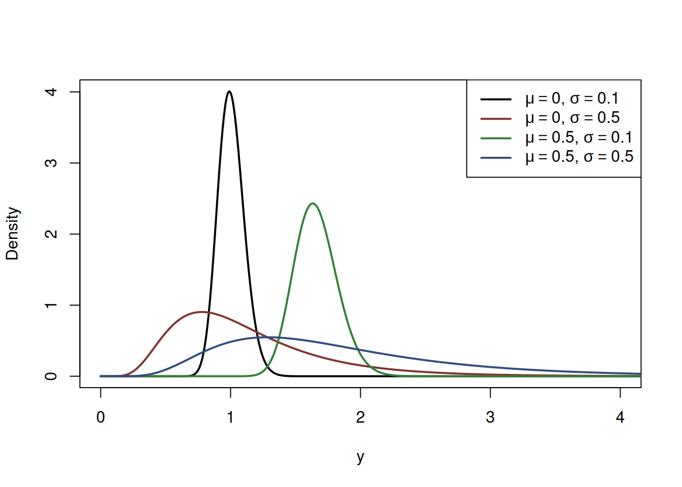
Figure 4.16: Probability Density Function of Log-Normal distribution with a variety of parameters.
The Figure 4.16 shows that with the increase of the location parameter \(\mu\), the distribution shifts to the right, while with the increase of the scale parameter \(\sigma\) it becomes more asymmetric with a longer right tail and its mode moves closer to zero. In fact, the skewness of the Log-Normal distribution depends solely on the value of \(\sigma^2\) - the higher it is, the more skewed the distribution is. It can be calculated as: \[\begin{equation} \mathrm{Sk}(y) = \left(e^{\sigma^2} + 2\right) \sqrt{e^{\sigma^2}-1} . \tag{4.13} \end{equation}\]
Log-Normal distribution is supported by dlnorm(), plnorm(), qlnorm() and rlnorm() functions from stats package in R.