4.5 Exponential distribution
We have already touched upon the Exponential distribution, when we discussed the arrival times in Poisson distribution (Section 3.5). Exponential distribution is used in modelling time between arrivals, because it is memoryless. We mentioned earlier that if a process is memoryless, then the following holds: \[\begin{equation*} \mathrm{P}(t > \tau_1 + \tau_2) = \mathrm{P}(t > \tau_1)\mathrm{P}(t > \tau_2) . \end{equation*}\] Exponential distribution relies on this property. It has only one parameter, the rate \(\lambda\) and can be written as \(\mathcal{Exp}(\lambda)\). Here is its PDF: \[\begin{equation} f(t, \lambda) = \lambda e^{-\lambda t} , \tag{4.14} \end{equation}\] where \(t\) is a positive number and \(\lambda\) is the rate parameter. This PDF is shown in Figure 4.17.
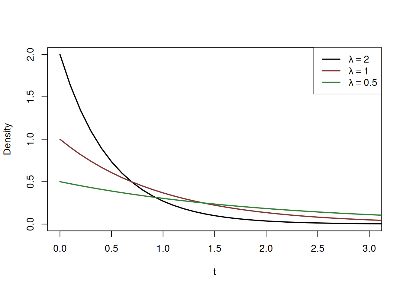
Figure 4.17: Probability Density Function of Exponential distribution with several values of rate parameter \(\lambda\).
The plot in Figure 4.17 shows that there is more likely for the variable \(t\) to get lower values (closer to zero) than the higher ones. The parameter \(\lambda\) controls the steepness of decline of the density curve with increase of \(t\): the higher the rate is, the more likely it is that the event will occur earlier and less likely that it will occur later.
The CDF of the distribution is shown in Figure 4.18.
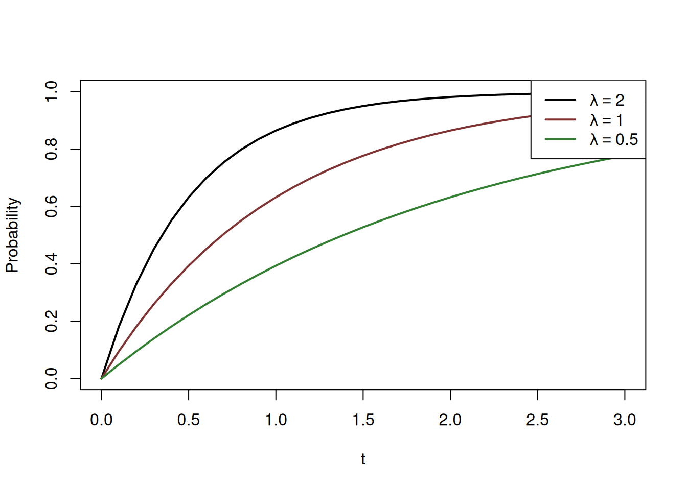
Figure 4.18: Cumulative Distribution Function of Exponential distribution with a variety of rate parameters.
The CDFs show how fast the probability of one is achieved with different rates. Mathematically, it is written as: \[\begin{equation} \mathrm{F}(t, \lambda) = 1 - e^{- \lambda t}. \tag{4.15} \end{equation}\] Based on it, we can say, for example what is the probability that an event will occur in 1.5 seconds if the rate is \(\lambda=2\) per second. It is: \[\begin{equation*} \mathrm{F}(t < 1.5, 2) = 1 - e^{- 2 \times 1.5} \approx 0.95 . \end{equation*}\]
This can also be calculated in R:
## [1] 0.9502129Coming back to the memorylessness property of the distribution, in order to show it visually, consider an example based on the property: \[\begin{equation*} \mathrm{P}(t > 1.5) = \mathrm{P}(t > 0.5) \mathrm{P}(t > 1) \end{equation*}\] and \(\lambda=2\). Note that \(P(t>a)=1-F(a)\) by definition of CDF. In terms of probabilities of Exponential distribution, this means that: \[\begin{equation*} \mathrm{P}(t > 1.5) = (1-\mathrm{F}(1, 2)) (1-\mathrm{F}(0.5, 2)) . \end{equation*}\] Now, in order to show this property visually, we take logarithms of the left and right hand sides of the previous equation to get: \[\begin{equation} \log \left( \mathrm{P}(t > 1.5) \right) = \log \left(1-\mathrm{F}(1, 2) \right) + \log \left( 1-\mathrm{F}(0.5, 2) \right) . \tag{4.16} \end{equation}\] We take logarithms to linearise relation, because it is easier to work with. If we now insert (4.15) in (4.16), we will get: \[\begin{equation} \log \left( \mathrm{P}(t > 1.5) \right) = \log \left(1- 1 + e^{- 2 \times 1} \right) + \log \left(1- 1 + e^{- 2 \times 0.5} \right) = -2 - 1 = -3 , \tag{4.17} \end{equation}\] which is obtained independently for \(\log(1-F(1.5, 2))=\log(e^{-2 \times 1.5})=-3\). We can also plot the function \(\log(1-F(t, 2))\) in Figure 4.19 to show that (4.17) holds, when the values on y-axis are added.
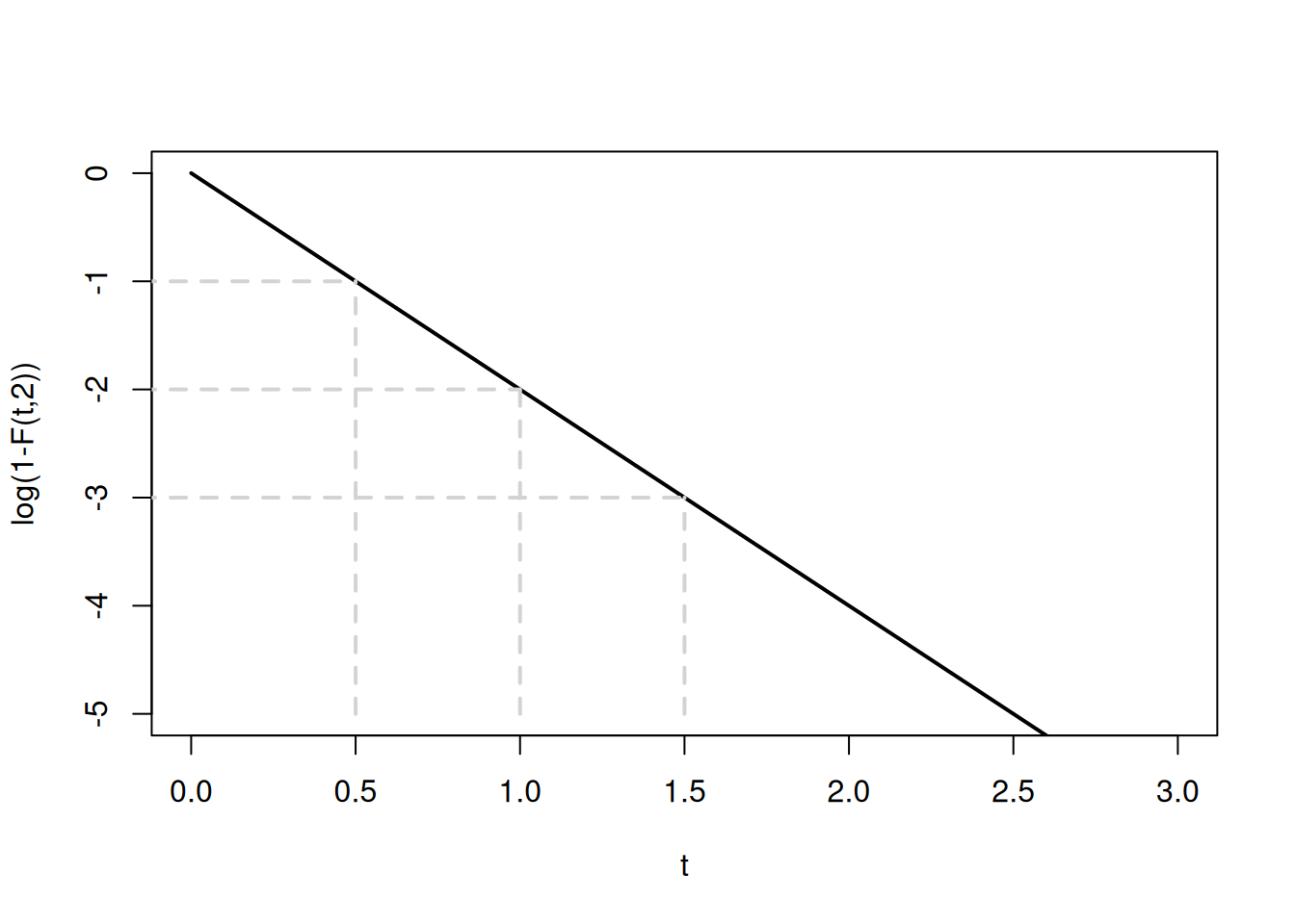
Figure 4.19: Memoryless property of Exponential distibution with \(\lambda=2\).
Note that because of the logarithm of the CDF, the function has now become linear, and the property becomes more apparent.
When it comes to the mean of the distribution, it is equal to: \[\begin{equation} \mathrm{E}(t) = \frac{1}{\lambda}, \tag{4.18} \end{equation}\] which makes it easy to estimate on a sample of observations – just take the mean, and you get an estimate of the rate parameter \(\lambda\). Furthermore, the rate parameter in Exponential distribution is directly related to the one in the Poisson (Section 3.5): the parameter in the latter equals the ratio of time interval \(t\) and \(\lambda\): \[\begin{equation} \lambda_P = \frac{t}{\lambda}, \tag{4.19} \end{equation}\] where \(\lambda_P\) is the parameter of the Poisson distribution. The main difference between the distributions is that Poisson explains the number of arrivals over a fixed period of time, while the Exponential represents the time between the arrivals.
Finally, the variance in Exponential distribution is calculated as: \[\begin{equation} \mathrm{V}(t) = \frac{1}{\lambda^2}, \tag{4.20} \end{equation}\]
In R, the Exponential distribution is implemented in dexp(), pexp(), qexp() and rexp() for PDF, CDF, QF and Random variables respectively.