13.2 Categorical variables for the slope
In reality, we can have more complicated situations when the change in costs of different types of properties would lead to the different overall costs. Visually, this would imply different slopes for the regression lines for the scatterplots for different properties types. Figure 13.6 demonstrates this idea with the three lines going through the cloud of points for the three property types.
# The general plot
plot(SBA_Chapter_11_Costs[,c("materials","overall")])
# Plot for the detached houses
points(SBA_Chapter_11_Costs[house_types[,1]==1,c("materials","overall")],
       pch=16, col=2)
# We added LOWESS lines to see whether the relations change
lm(overall~materials,
   SBA_Chapter_11_Costs[house_types[,1]==1,]) |>
  abline(col=2)
# Semi-detached
points(SBA_Chapter_11_Costs[house_types[,2]==1,c("materials","overall")],
       pch=16, col=3)
lm(overall~materials,
   SBA_Chapter_11_Costs[house_types[,2]==1,]) |>
  abline(col=3)
# Other
points(SBA_Chapter_11_Costs[house_types[,3]==1,c("materials","overall")],
       pch=16, col=4)
lm(overall~materials,
   SBA_Chapter_11_Costs[house_types[,3]==1,]) |>
  abline(col=4)
# Create the legend for convenience
legend("topleft", legend=levels(SBA_Chapter_11_Costs$type),
       col=c(2,3,4), lwd=1, pch=16)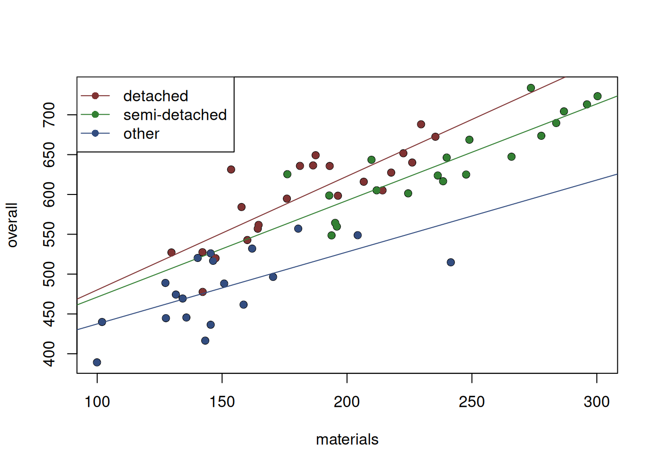
Figure 13.6: Scatterplot of material vs overall costs for the three property types.
It becomes apparent from the Figure that the lines have different slopes, and thus in our model we should take this into account. In this case, we are talking about an interaction effect between the type and material costs. While we could fit three models to address this, there is a more elegant solution involving the dummy variables. All we need to do is to multiply the materials variable with each of the dummy variables. And because the dummy variables take only values of zero and one, the newly created variables will have either the original value, or zero:
materialsTypes <- SBA_Chapter_11_Costs$materials * house_types
colnames(materialsTypes) <- paste0("mat_", colnames(house_types))
# Bind columns and show the first 7 rows
cbind(materials=SBA_Chapter_11_Costs$materials,
      house_types,
      materialsTypes) |> head(7)
## materials typedetached typesemi-detached typeother mat_typedetached
## 1 131.50 0 0 1 0.00
## 3 217.68 1 0 0 217.68
## 4 162.03 0 0 1 0.00
## 5 192.88 0 1 0 0.00
## 6 146.40 0 0 1 0.00
## 7 193.82 0 1 0 0.00
## 8 160.10 1 0 0 160.10
## mat_typesemi-detached mat_typeother
## 1 0.00 131.50
## 3 0.00 0.00
## 4 0.00 162.03
## 5 192.88 0.00
## 6 0.00 146.40
## 7 193.82 0.00
## 8 0.00 0.00The output above shows how the newly created variables look. For example, the mat_typedetached contains zero in the first row because the dummy variable typedetached equals to zero for that observation. But when it comes to the second one, it equals 217.68 because the respective dummy variable equals to one and 217.68$$1=217.68. Now having introduced these interaction variables, we can include them in the regression model and the estimated parameters would capture the specific effects of materials costs on the overall costs for each of the property types.
In R, if we deal with the categorical variable, we can introduce the effects via the formula by using the colon symbol (“:”):
costsModelInteraction <- alm(overall~size+materials:type+projects+year,
                             SBA_Chapter_11_Costs)
summary(costsModelInteraction)
## Response variable: overall
## Distribution used in the estimation: Normal
## Loss function used in estimation: likelihood
## Coefficients:
## Estimate Std. Error Lower 2.5% Upper 97.5%
## (Intercept) -2765.8065 3154.3285 -9092.5884 3560.9753
## size 0.9305 0.5928 -0.2586 2.1195
## projects -5.4693 2.7892 -11.0638 0.1252
## year 1.5470 1.5719 -1.6058 4.6998
## materials:typedetached 1.0881 0.2258 0.6353 1.5410 *
## materials:typesemi-detached 0.8763 0.2347 0.4055 1.3471 *
## materials:typeother 0.6270 0.2254 0.1748 1.0792 *
##
## Error standard deviation: 31.1051
## Sample size: 61
## Number of estimated parameters: 8
## Number of degrees of freedom: 53
## Information criteria:
## AIC AICc BIC BICc
## 599.8943 602.6635 616.7813 622.4733The output above now has rows materials:typedetached and others, which capture the specific effects.