8.1 One-sample tests about mean
Consider an example, where we collected the data of height of 100 males across England for the 2021. Based on that sample we want to see if the average height is 175.3 cm, as it was claimed by NHS back in 2012. Based on our sample, we found that the mean height was 176.1 cm. Can we say that the height has increased or did we get this value just because of the pure randomness? How do we formulate and test such hypothesis? We need to follow the procedure described in Section 7.1. We start by formulating null and alternative hypotheses: \[\begin{equation*} \mathrm{H}_0: \mu = 175.3, \mathrm{H}_1: \mu \neq 175.3 . \end{equation*}\] Next, we select the significance level. If the level is not given to us, then we need to choose one based on our preferences. I like 1%, because I am risk averse.
After that, we select the appropriate test. The task described above focuses on investigating the hypothesis about the mean. If we can assume that the CLT holds (see Section 6.3), then we can use a parametric statistical test, because we know that the sample mean will follow Normal distribution in that case. In our example, we can indeed assume that it holds, because we deal with a sample of 100 observations, and we can also assume that the distribution of height across England is symmetric (we do not expect people to have extreme heights of, let’s say, 5 meters or 0.5 meters). The next thing to consider is whether the population standard deviation of the mean height is known or not. Based on that, we would choose either z-test or t-test.
8.1.1 z-test
Consider the situation, where we know from NHS that the population standard deviation of height is \(\sigma=5\) (typically, we do not know it, except for some very rare cases, when this is given by design, e.g. due to how some machine is calibrated).
Remark. As shown in Section 6.5, if the standard deviation of \(y\) is \(\sigma\), then the standard deviation of \(\bar{y}\) is \(\frac{1}{\sqrt{n}} \sigma\). This means that in our case \(\sigma_{\bar{y}}=\frac{1}{\sqrt{100}} \times 5 =0.5\).
If we assume that the mean follows Normal distribution and know the population standard deviation, i.e. \(\bar{y} \sim \mathcal{N}\left(\mu, \sigma^2_{\bar{y}}\right)\), then the standardised value z: \[\begin{equation} z = \frac{\bar{y}-\mu}{\sigma_{\bar{y}}} . \tag{8.1} \end{equation}\] will follow standard normal distribution: \(z \sim \mathcal{N}\left(0, 1\right)\). Knowing these properties, we can conduct the test using one of the three approaches discussed in Section 7.1. First, we could calculate the z value based on formula (8.1): \[\begin{equation*} z = \frac{176.1 -175.3}{0.5} = 1.6 \end{equation*}\] and compare it with the critical one. Given that we test the two-sided hypothesis (because the alternative is “inequality”), he critical value should be split into two parts, to have \(\frac{\alpha}{2}\) in one tail and \(\frac{\alpha}{2}\) in the other one. The critical values can be calculated, for example, in R using the code below:
# I have previously selected significance level of 1%
alpha <- 0.01
qnorm(c(alpha/2, 1-alpha/2), 0, 1)
## [1] -2.575829 2.575829We see that the calculated value lies inside the interval, so we fail to reject the null hypothesis on 1% significance level. The simplified version for this procedure is to compare the absolute of the calculated value with the absolute of the critical one. If the calculated is greater than the critical, then we reject H\(_0\). In our case 1.6 < 2.58, so we fail to reject H\(_0\).
Another way of testing the hypothesis is by calculating the p-value and comparing it with the significance level. In R, this can be done using the command:
## [1] 0.1095986In the R code above we are calculating the surface in the tails of distribution. Thus the appearance of the number 2, to add the surfaces in two tails. This procedure is shown in Figure 8.1.
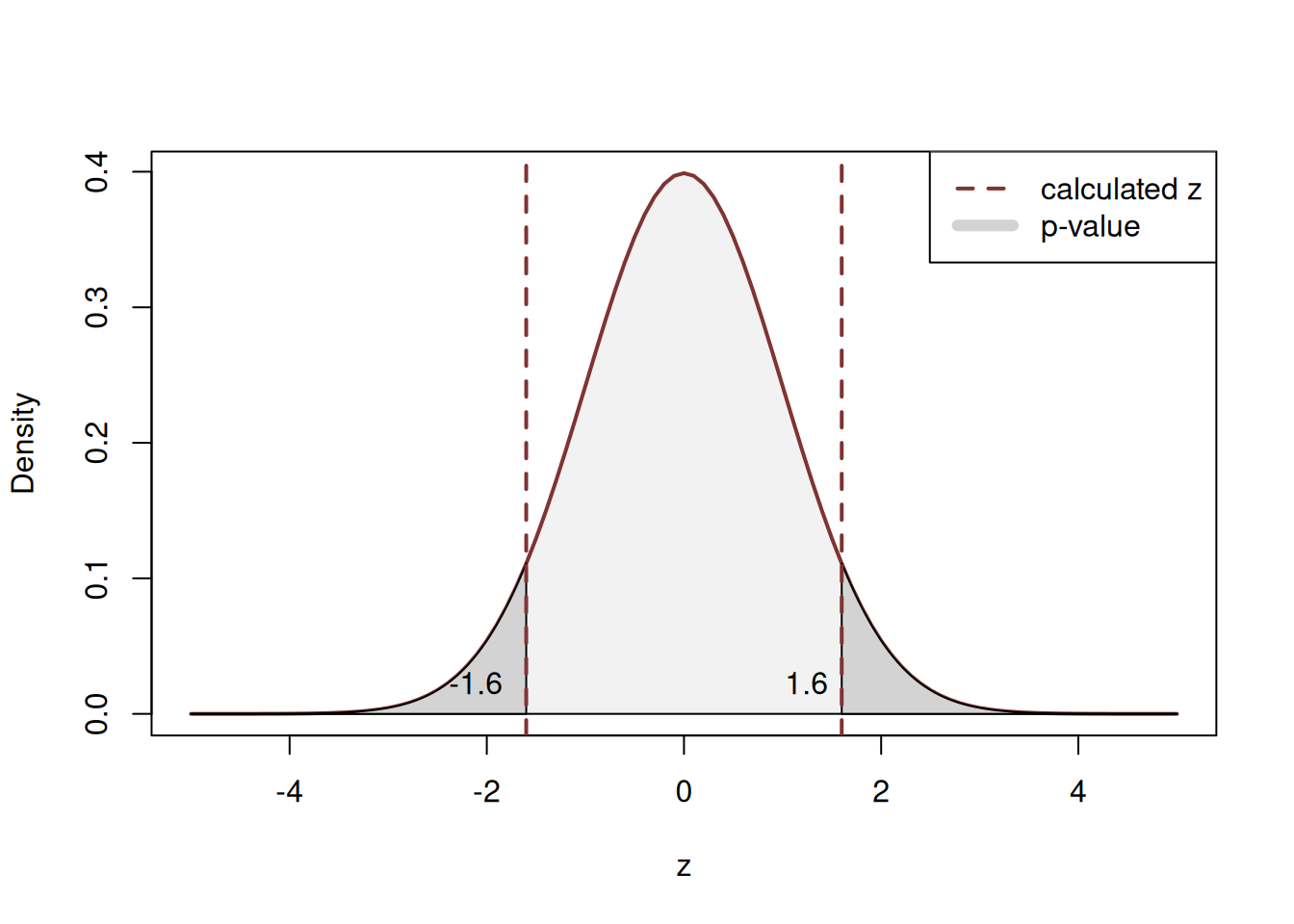
Figure 8.1: The process of p-value calculation for the z-test.
Comparing the p-value of 0.1096 with the significance level of 0.01, we can conclude that we fail to reject the null hypothesis. This means that based on the collected sample, we cannot tell the difference between the population mean height of 175.3 and the sample height of 176.1.
8.1.2 t-test
The population standard deviation is rarely known. The more practical test is the t-test, which relies on the relation between the normal distribution and the Student’s distribution. If \(y \sim \mathcal{N}(\mu ,\sigma^2)\) and \(s=\sqrt{\frac{1}{n}\sum_{j=1}^n{\left(y_j-\bar{y}\right)^2}}\) is the estimate of the sample standard deviation, then \(t \sim \mathcal{t}(n-1)\) where \[\begin{equation} t = \frac{\bar{y}-\mu}{s_{\bar{y}}} \tag{8.2} \end{equation}\] and \(n-1\) is the number of degrees of freedom. The reason why we need to use Student’s distribution in this case rather than the Normal one is because of the uncertainty arising from the estimation of the standard deviation \(s\). The hypothesis testing procedure in this case is exactly the same as in the case of z-test. We insert the values in (8.2) to get the calculated t, then compare it with the critical and make a conclusion. Consider an example, where the estimated standard deviation \(s=4\). We then get: \[\begin{equation*} t = \frac{176.1-175.3}{0.4} = 2 , \end{equation*}\] while the critical value for the chosen 1% significance level is:
## [1] -2.626405 2.626405Given that the calculated value of 2 is lower than 2.626, we fail to reject the null hypothesis on 1% significance level. So, we again conclude that we cannot tell the difference between the mean in the data and the assumed population mean.
In R, the same procedures can be done using the t.test() function from stats package. Here is an example, demonstrating how the test can be done for the generated data:
y <- rnorm(100, 175.3, 5)
# Note that our significance level is 1%,
# so we ask to produce 99% confidence interval
t.test(y, mu=175.3, alternative="two.sided", conf.level=0.99)
##
## One Sample t-test
##
## data: y
## t = 1.8509, df = 99, p-value = 0.06717
## alternative hypothesis: true mean is not equal to 175.3
## 99 percent confidence interval:
## 174.9013 177.6018
## sample estimates:
## mean of x
## 176.2516Remark. If we were to test a one-sided hypothesis (e.g. \(\mathrm{H}_0: \mu \leq 175.3, \mathrm{H}_1: \mu > 175.3\)), then we would need to change the alternative parameters in the t.test() function to correspond to the formulated H\(_1\).
The output above shows the calculated t (1.8509), the number of degrees of freedom and the p-value. It also constructs the 99% confidence interval (174.9013, 177.6018). The conclusions can be made using one of the three approaches, discussed above and in Section 7.1:
- The calculated value is 1.8509, which is lower than the critical one of 2.6264 as discussed earlier, so we fail to reject H\(_0\);
- The p-value is 0.0672, which is greater than the selected significance level of 1%, so we fail to reject H\(_0\);
- The 99% confidence interval includes the tested value of 175.3, so we fail to reject the H\(_0\) on the 99% confidence level.
As mentioned in Section 7.1, I personally prefer the last approach of the three because it gives more information about the uncertainty around the estimate of the sample mean.
8.1.3 Non-parametric, one-sample Wilcoxon test
In some situations, the CLT might not hold due to violation of some of assumptions. For example, the distribution of the random variable is expected to be asymmetric with a long tail. In this case, the mean might not be finite and thus the CLT would not hold. Alternatively, the sample size might be too small to assume that CLT has started working. In these cases, the parametric tests for the mean will not be powerful enough (see discussion in Section 7.3) and would lead to wrong conclusions about the tested hypothesis.
One of the solutions in this situation is a non-parametric test that does not have distributional assumptions. In the case of the hypothesis about the mean of a random variable, we could use Wilcoxon test. The null hypothesis in this test can be formulated in a variety of ways, one of which is the following: \[\begin{equation*} \begin{aligned} &\mathrm{H}_0: \text{ distribution is symmetric around } \mu = 175.3, \\ &\mathrm{H}_1: \text{ distribution is not symmetric around } \mu = 175.3 . \end{aligned} \end{equation*}\] If the H\(_0\) is true in this case, then it means that the mean will coincide with the centre of distribution, which should be around the tested value. If it is not symmetric, then possibly the centre of distribution is not around the tested value. The test is done on the ranked data, sorting the values of \(y\) from the lowest to the highest and assigning the numerical values to them. After that the test values is calculated.
Given that the test does not rely on distributional assumptions, it is less powerful than the parametric tests on large samples, but it is also more powerful on the small ones.
In R, the test can be conducted using wilcox.test() function from stats package:
##
##  Wilcoxon signed rank test with continuity correction
##
## data:  y
## V = 3039, p-value = 0.07747
## alternative hypothesis: true location is not equal to 175.3
Similar to how we have done that with t-test, we can compare the p-value with the significance level (reminder: we have chosen 1%) and make a conclusion. Based on the output above, we fail to reject H\(_0\) because 0.0775>0.01.This means that once again, we cannot tell the difference between the sample mean and the population mean of 175.3.