3.6 Discrete Uniform distribution (Rolling a dice)
In the second world war, the UK faced a problem of understanding how many tanks Nazi Germany had. Some tank components had serial numbers, and when some of tanks were captured or destroyed, it was possible to track these numbers. But was it possible to say how many enemy tanks there were overall? As it appears, it was. From the stand point of the UK, it was equally possible to have a serial number 0001, 0042, 0500 or, say, 1984. The distribution of these serial numbers could be assumed uniform, which was then used to get an estimate of the maximum number of tanks that the enemy had. We will come back to the solution of this problem at the end of this section.
This distribution is one of the basic ones in the probability theory. For now we focus on the discrete version of it, keeping in mind that there also exists the continuous one (see Section 4.2).
The classical example of application of this distribution is dice rolling. The conventional dice has 6 sides and when rolled can give a value of 1 to 6. If the dice is fair then the probability of getting a score on it is the same for all the sides. This means that the PMF of the distribution can be written as: \[\begin{equation} f(y, k) = \frac{1}{k}, \tag{3.16} \end{equation}\] where \(k\) is the number of outcomes (sides of the dice). The more outcomes there are, the lower the probability of having a specific outcome is. For example, on a dice with 10 sides, the probability of getting the score 5 is \(\frac{1}{10}\), while on the 6-sided version it is \(\frac{1}{6}\).
The PMF of the Uniform distribution is shown visually in Figure 3.9 on example of 1d6.
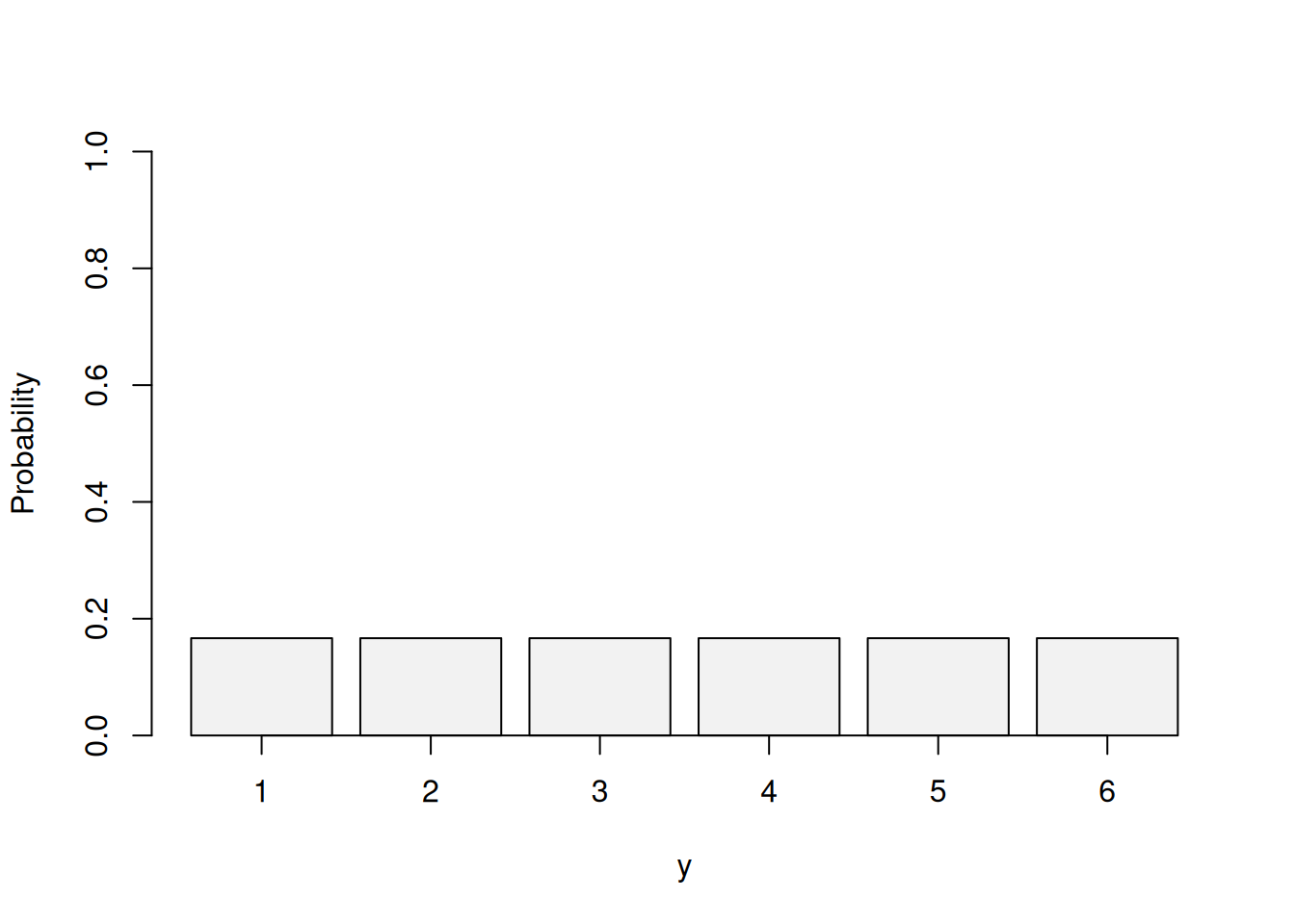
Figure 3.9: Probability Mass Function of Uniform distribution for 1d6.
The mean of this distribution is calculated as \(\frac{a+b}{2}\), where \(a\) is the lowest and \(b\) is the highest possible values. So, for the 1d6, the mean is \(\frac{1+6}{2}=3.5\). This means that if we roll the dice many times the average score will be 3.5.
The variance of the uniform distribution depends on the number of outcomes and is calculated as: \[\begin{equation} \sigma^2(y, k) = \frac{k^2-1}{12} . \tag{3.17} \end{equation}\] As can be seen from the formula, the variance of Uniform distribution is proportional to the number of outcomes.
Coming to the CDF of the Uniform distribution, it is calculated as: \[\begin{equation} f(y, k) = \frac{y-a+1}{k}, \tag{3.18} \end{equation}\] where \(a\) is the lowest possible value and \(k\) is the number of outcomes. This CDF can be visualised as shown in Figure 3.10.
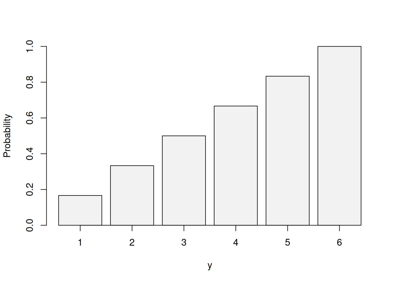
Figure 3.10: Cumulative Distribution Function of Uniform distribution for 1d6.
Given that the probability of each separate outcome in the Uniform distribution is always \(\frac{1}{k}\), the CDF demonstrates a linear growth, reaching 1 at the highest point, which can be interpreted as rolling 1d6, we will always get a value up to 6 (less than or equal to 6). The CDF can be used to get probabilities of several events at the same time. For example, we can say that when rolling 1d6 the probability of getting 1 or 2 is \(\frac{2-1+1}{6}=\frac{1}{3}\).
Bernoulli distribution (Section 3.3) with \(p=0.5\) can be considered as a special case of the Uniform distribution (with only two outcomes).
A company produces headphones, putting serial numbers on them. So far, it has produced 9,990 of them. If a customer buys headphones, what is the probability that they will get a serial number with three digits?
Solution. This is the task on Uniform distribution, because serial numbers do not repeat and we can assume that the probability of getting any of them is the same. In terms of parameters, \(a=1\) and \(b=9990\). To get a serial number with three digits, a customer needs to have anything between 100 and 999. This can be formulated as: \[\begin{equation*} \mathrm{P}(100 \leq y \leq 999) = \mathrm{P}(y \leq 999) - \mathrm{P}(y \leq 99). \end{equation*}\] Inserting the values in the CDF of the Uniform distribution (3.18) we get: \[\begin{equation*} \mathrm{P}(100 \leq y \leq 999) = \frac{999}{9990} - \frac{99}{9990} \approx 0.1 - 0.01 = 0.09. \end{equation*}\]
Remark. Similarly how Binomial distribution is a generalisation of the Bernoulli, there is distribution describing the multiple dice rolls. It is called the Multinomial distribution. While we do not discuss it here, we note that this is a distribution, which is, for example, used to model respondents choices in survey, when the variable of interest is in a categorical scale and the probabilities for different options are not equal.
Coming back to the example with the German tanks, this problem was solved by estimating the maximum of the uniform distribution, i.e. getting the estimate of \(b\). Goodman (1952) provides a solution. He showed how to find the maximum for a set of serial numbers. An unbiased and efficient estimate of the maximum value can be calculated using the following formula: \[\begin{equation*} \hat{b} = m + \frac{m}{k}-1, \end{equation*}\] where \(m\) is the maximum number observed in the sample, and \(k\) is the number of the observed values. For the sequence of serial numbers (from Goodman, 1954) 83, 135, 274, 380, 668, 895, 955, 964, 1113, 1174, 1210, 1344, 1387, 1414, 1610, 1668, 1689, 1756, 1865, 1874, 1880, 1936, 2005, 2006, 2065, 2157, 2220, 2224, 2396, 2543 and 2787, we have: \[\begin{equation*} \hat{b} = 2787 + \frac{2787}{31}-1 \approx 2876 . \end{equation*}\] The real maximum number in that example was 2885, making the estimate above quite accurate. There are several solutions to this problem, and in the Second World War, statistical estimates were shown to be much more accurate than the ones obtained via intelligence.