14.2 Types of variables transformations
Having considered this case study, we can summarise the possible types of transformations of variables in regression models and what they would mean. Here, we only discuss monotonic transformations, i.e. those that guarantee that if \(x\) was increasing before transformations, it would be increasing after transformations as well.
14.2.1 Linear model
\[\begin{equation} y = \beta_0 + \beta_1 x + \epsilon . \tag{14.10} \end{equation}\]
As discussed earlier, in this model, \(\beta_1\) can be interpreted as a marginal effect of x on y. The typical interpretation is that with the increase of \(x\) by 1 unit, \(y\) will change on average by \(\beta_1\) units. In case of dummy variables, their interpretation is that the specific category of product will have a different (higher or lower) impact on \(y\) by \(\beta_1\) units. e.g. “sales of red mobile phones are on average higher than the sales of the blue ones by 100 units”.
14.2.2 Log-Log model
Or power model or a multiplicative model: \[\begin{equation} \log y = \beta_0 + \beta_1 \log x + \log (1+\epsilon) . \tag{14.11} \end{equation}\] It is equivalent to \[\begin{equation} y = \beta_0 x^{\beta_1} (1+\epsilon) . \tag{14.12} \end{equation}\] The parameter \(\beta_1\) is interpreted as elasticity: If \(x\) increases by 1%, the response variable \(y\) changes on average by \(\beta_1\)%. Depending on the value of \(\beta_1\), this model can capture non-linear relations with slowing down or accelerating changes. Figure 14.8 demonstrates several examples of artificial data with different values of \(\beta_1\).
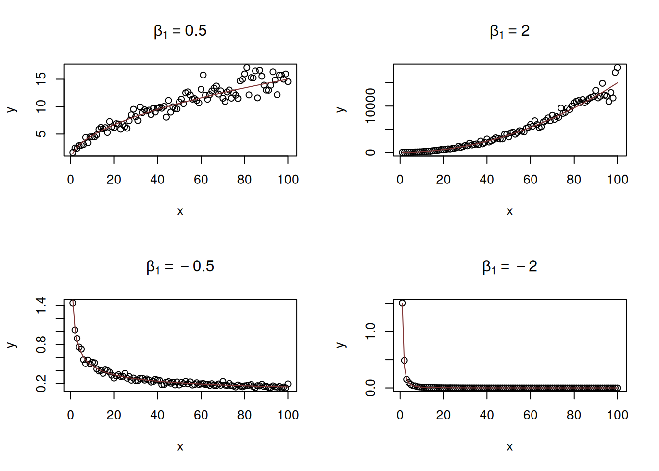
Figure 14.8: Examples of log-log relations with different values of elasticity parameter.
As discussed earlier, this model can only be applied to positive data. If there are zeroes in the data, then logarithm will be equal to \(-\infty\) and it would not be possible to estimate the model correctly.
14.2.3 Log-linear model
Or exponential model: \[\begin{equation} \log y = \beta_0 + \beta_1 x + \log (1+\epsilon) . \tag{14.13} \end{equation}\] is equivalent to \[\begin{equation} y = \beta_0 \exp(\beta_1 x) (1+\epsilon) . \tag{14.14} \end{equation}\]
The parameter \(\beta_1\) will control the change of speed of growth / decline in the model. If variable \(x\) increases by 1 unit, then the variable \(y\) will change on average by \((\exp(\beta_1)-1)\times 100\)%. If the value of \(\beta_1\) is small (roughly \(\beta_1 \in (-0.2, 0.2)\)), then due to one of the limits the interpretation can be simplified to: when \(x\) increases by 1 unit, the variable \(y\) will change on average by \(\beta_1\times 100\)%. The exponent is in general a dangerous function as it exhibits either explosive (when \(\beta_1 > 0\)) or implosive (when \(\beta_1 < 0\)) behaviour. This is shown in Figure 14.9, where the values of \(\beta_1\) are -0.05 and 0.05, and we can see how fast the value of \(y\) changes with the increase of \(x\).
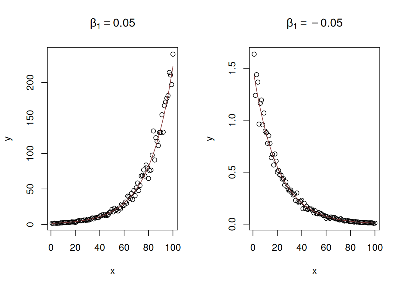
Figure 14.9: Examples of log-linear relations with two values of slope parameter.
If \(x\) is a dummy variable (see Section 13), then its interpretation is slightly different: the presence of the effect \(x\) leads on average to the change of variable \(y\) by \(\beta_1 \times 100\)%. e.g. “sales of red laptops are on average 15% higher than sales of blue laptops”.
14.2.4 Linear-Log model
Or logarithmic model. \[\begin{equation} y = \beta_0 + \beta_1 \log x + \epsilon . \tag{14.15} \end{equation}\] This is just a logarithmic transform of explanatory variable. The parameter \(\beta_1\) in this case regulates the direction and speed of change. If \(x\) increases by 1%, then \(y\) will change on average by \(\frac{\beta_1}{100}\) units. Figure 14.10 shows two cases of relations with positive and negative slope parameters.
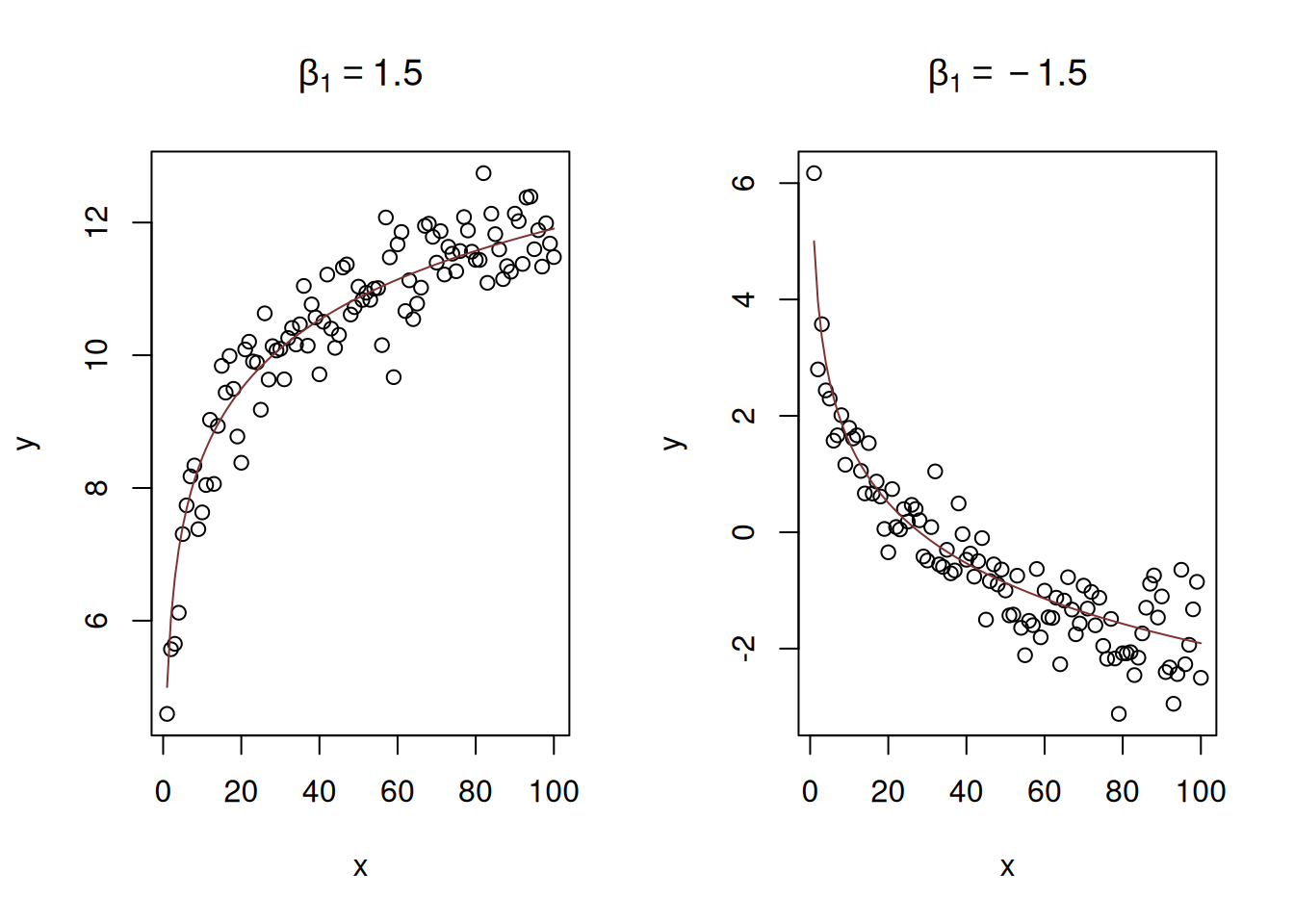
Figure 14.10: Examples of linear-log relations with two values of slope parameter.
The logarithmic model assumes that the increase in \(x\) always leads on average to the slow down of the value of \(y\).
14.2.5 Square root model
\[\begin{equation} y = \beta_0 + \beta_1 \sqrt x + \epsilon . \tag{14.16} \end{equation}\] The relation between \(y\) and \(x\) in this model looks similar to the on in linear-log model, but the with a lower speed of change: the square root represents the slow down in the change and might be suitable for cases of diminishing returns of scale in various real life problems. There is no specific interpretation for the parameter \(\beta_1\) in this model - it will show how the response variable \(y\) will change on average wih increase of square root of \(x\) by one. Figure 14.11 demonstrates square root relations for two cases, with parameters \(\beta_1=1.5\) and \(\beta_1=-1.5\).
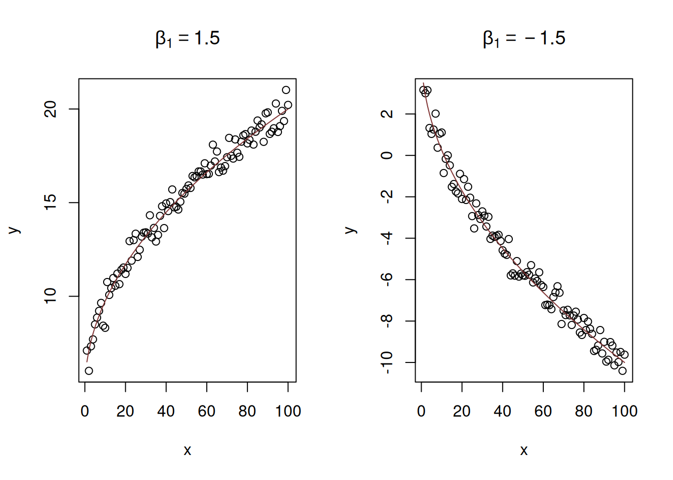
Figure 14.11: Examples of linear - square root relations with two values of slope parameter.
14.2.6 Quadratic model
\[\begin{equation} y = \beta_0 + \beta_1 x + \beta_2 x^2 + \epsilon . \tag{14.17} \end{equation}\] This relation demonstrates increase or decrease with an acceleration due to the present of squared \(x\). This model has an extremum (either a minimum or a maximum), when \(x=\frac{-\beta_1}{2 \beta_2}\). This means that the growth in the data will be changed by decline or vice versa with the increase of \(x\). This makes the model potentially prone to overfitting, so it needs to be used with care. Note that in general the quadratic equation should include both \(x\) and \(x^2\), unless we know that the extremum should be at the point \(x=0\) (see the example with Model 5 in the previous section). Furthrmore, this model is close to the one with square root of \(y\): \(\sqrt y = \beta_0 + \beta_1 x + \epsilon\), with the main difference being that the latter formulation assumes that the variability of the error term will change together with the change of \(x\) (so called “heteroscedasticity” effect, see Section 15.2). This model was used in the examples with stopping distance above. Figure 14.12 shows to classical examples: with branches of the function going down and going up.
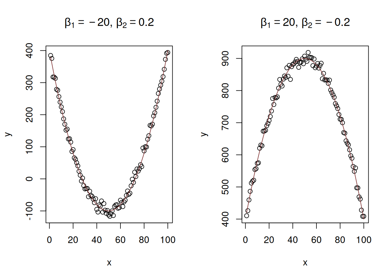
Figure 14.12: Examples of linear-log relations with two values of slope parameter.
14.2.7 Polynomial model
\[\begin{equation} y = \beta_0 + \beta_1 x + \beta_2 x^2 + \dots \ \beta_k x^k + \epsilon . \tag{14.18} \end{equation}\] This is a more general model than the quadratic one, introducing \(k\) polynomials. This is not used very often in analytics, because any data can be approximated by a high order polynomial, and because the branches of polynomial will inevitably lead to infinite increase / decrease, which is not a common tendency in practice.
14.2.8 Box-Cox transform
Or power transform: \[\begin{equation} \frac{y^\lambda -1}{\lambda} = \beta_0 + \beta_1 x + \epsilon . \tag{14.19} \end{equation}\] This type of transform can be applied to either response variable or any of explanatory variables and can be considered as something more general than linear, log-linear, quadratic and square root models. This is because with different values of \(\lambda\), the transformation would revert to one of the above. For example, with \(\lambda=1\), we end up with a linear model, just with a different intercept. If \(\lambda=0.5\), then we end up with square root, and when \(\lambda \rightarrow 0\), then the relation becomes equivalent to logarithmic. The choice of \(\lambda\) might be a challenging task on its own, however it can be estimated via likelihood. If estimated and close to either 0, 0.5, 1 or 2, then typically a respective transformation should be applied instead of Box-Cox. For example, if \(\lambda=0.49\), then taking square root might be a preferred option.
14.2.9 Logistic transform
In some cases, the variable of interest might lie in a specific region, for example between 0 and 100. In that case a non-linear transform is required to change the range to the conventional one \((-\infty, \infty)\) used in the classical regression. The logistic transform is supposed to do that. Assuming that \(y \in (0,1)\) the model based on it can be written as: \[\begin{equation} y = \frac{1}{1+\exp \left(-(\beta_0 + \beta_1 x + \epsilon)\right)}. \tag{14.20} \end{equation}\]
Remark. If \(y\) lies in a different fixed range, then a scaling can be applied to it to make it lie between zero and one. For example, if it lies between 0 and 100, division by 100 will fix the scale.
The inverse logistic transform might also be useful and allows estimating the model using the conventional methods after transforming the response variable: \[\begin{equation} \log \left( \frac{y}{1-y}\right) = \beta_0 + \beta_1 x + \epsilon. \tag{14.21} \end{equation}\]
The logistic function is used in models with binary response variable and is also one of the conventional functions used in more advanced machine learning techniques (e.g. Artificial Neural Networks). Figure ?? demonstrates how the response variable might look in the case of the model (14.20).
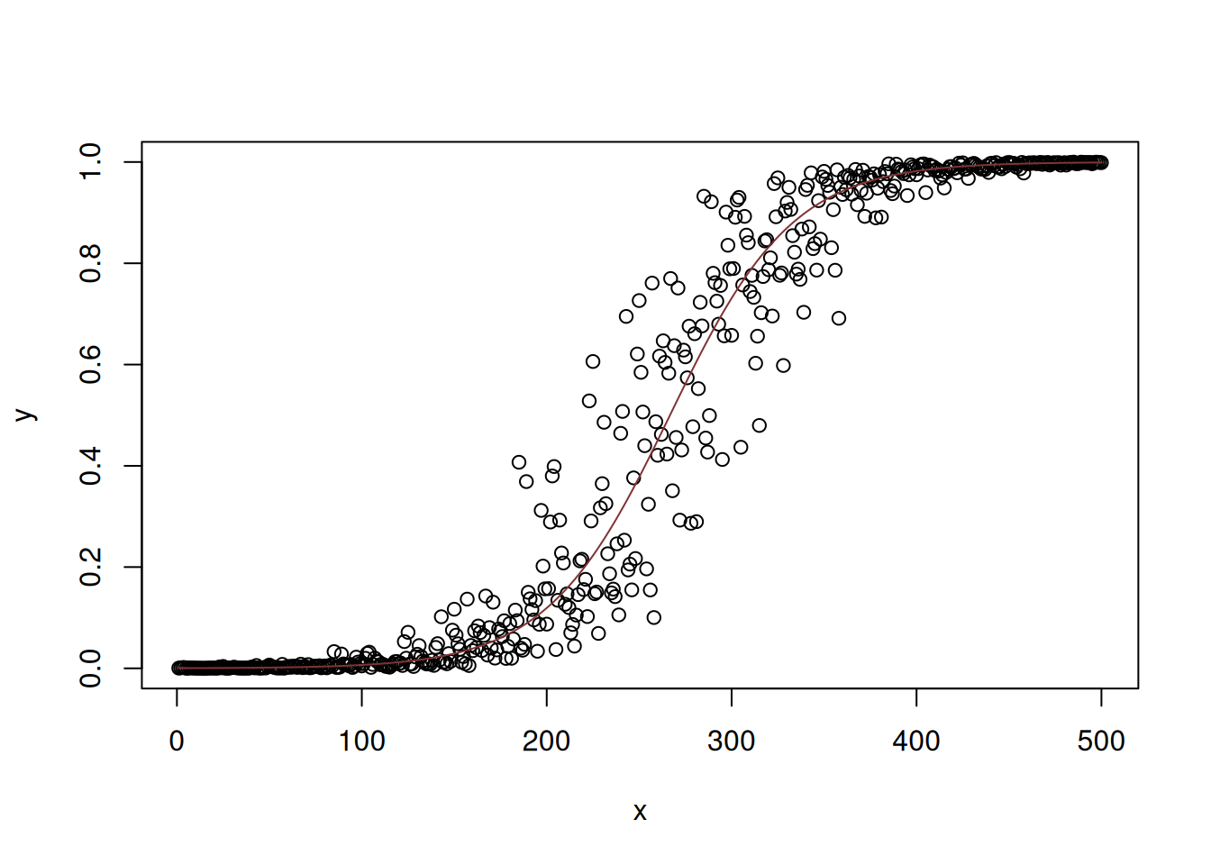
Figure 14.13: Examples of linear-log relations with two values of slope parameter.
Sometimes the value of \(y\) in case of logistic model is interpreted as a probability of outcome. We will discuss models based on logistic function later in this textbook.
14.2.10 Summary
In this subsection we discussed the basic types of variables transformations on examples with simple linear regression. The more complicated models with multiple explanatory variables and complex transformations can be considered as well. However, whatever transformation is considered, it needs to be meaningful and come from the theory, not from the data. Otherwise we may overfit the data, which will lead to a variety of issues, some of which are discussed in Section 15.1.