12.3 Regression line related uncertainty
Given the uncertainty of estimates of parameters, the regression line itself will vary with different samples. This means that in some cases we should not just consider the predicted values of the regression \(\hat{y}_j\), but should also consider the uncertainty around them.
Similar to what we discussed in Sections 6.5 and 6.6, there are two different interval types we can produce from the regression: confidence and prediction. It is extremely important to get the difference between the two, so here it is again just in case:
- Confidence interval shows where the expected value should lie in the population in the x% of the cases if we repeat the calculation for different samples of data many times;
- Prediction interval shows where the x% of the actual values should lie.
The former will tell you something about the true expected costs of a project, while the latter will tell you about the actual costs. The word “should” indicates that this is not necessarily always the case - the final outcome depends on the specific data (e.g. sample size) and the model (whether its assumptions hold).
12.3.1 Confidence interval
In the context of univariate statistics that we discussed in Section 6.5, the idea was to capture the uncertainty around the mean of the data. In case of regression, we are focusing on the conditional mean, i.e. the expected value, given the values of all explanatory variables for a specific observation. In the example that we have used in this chapter, this would come to understanding what the true expected overall costs should be, for example, for the material costs of 200 thousands of pounds, size of 90, 3 projects and the year 2008. This should be straight forward to calculate as long as we have the covariance matrix of parameters (Section 12.1).
The formula for the construction of the confidence interval is very similar to the one we discussed for the sample mean in Section 6.5: \[\begin{equation} \mu_j \in (\hat{y}_j + t_{\alpha/2}(n-k) s_{\hat{y}_j}, \hat{y}_j + t_{1-\alpha/2}(n-k) s_{\hat{y}_j}), \tag{12.14} \end{equation}\] where \(\mu_j\) is the true expectation, and \(s_{\hat{y}_j}=\sqrt{\mathrm{V}(\hat{y}_j| \mathbf{x}_j)}\) is the standard deviation of the fitted value. Compare this with the one we had in Section 6.5: \[\begin{equation*} \mu \in (\bar{y} + t_{\alpha/2}(n-1) s_{\bar{y}}, \bar{y} + t_{1-\alpha/2}(n-1) s_{\bar{y}}). \end{equation*}\] Here are the main differences:
- We now focus on \(\mu_j\), the expectation for a specific observation instead of just global average \(\mu\);
- We have the fitted value from the regression line \(\hat{y}_j\) instead of the sample mean \(\bar{y}\);
- We have the standard deviation of the line \(s_{\hat{y}_j}\) instead of the standard deviation of the mean \(s_{\bar{y}}\);
- We have \(n-k\) degrees of freedom instead of \(n-1\) because we estimated \(k\) parameters instead of just one (the sample mean).
But the rest is the same and uses exactly the same principles.
Remark. To be able to construct the confidence interval using the formula above, we, once again, need one important assumption to hold. This assumption is that the Central Limit Theorem holds (Section 6.3). If it does not, then the distribution of the estimates of parameters would not be Normal and as a result, the distribution of the conditional expectations would not be Normal either. In that case, we would need to use some other tools (such as bootstrap) to construct the interval. Luckily, with OLS, the CLT typically holds on samples of 50 observations and more.
In R, the confidence interval can be constructed for each observation via the predict() function with interval="confidence". It is based on the covariance matrix of parameters, extracted via vcov() method in R (discussed in Section 12.1). Note that the interval can be produced not only for the in-sample value, but for the holdout as well. Here is an example with alm() function (Figure 12.4):
# Produce predictions
costsModelMLRCI <- predict(costsModelMLR, interval="confidence")
plot(costsModelMLRCI, main="", type="p",
     xlab="Observation", ylab="Overall Costs")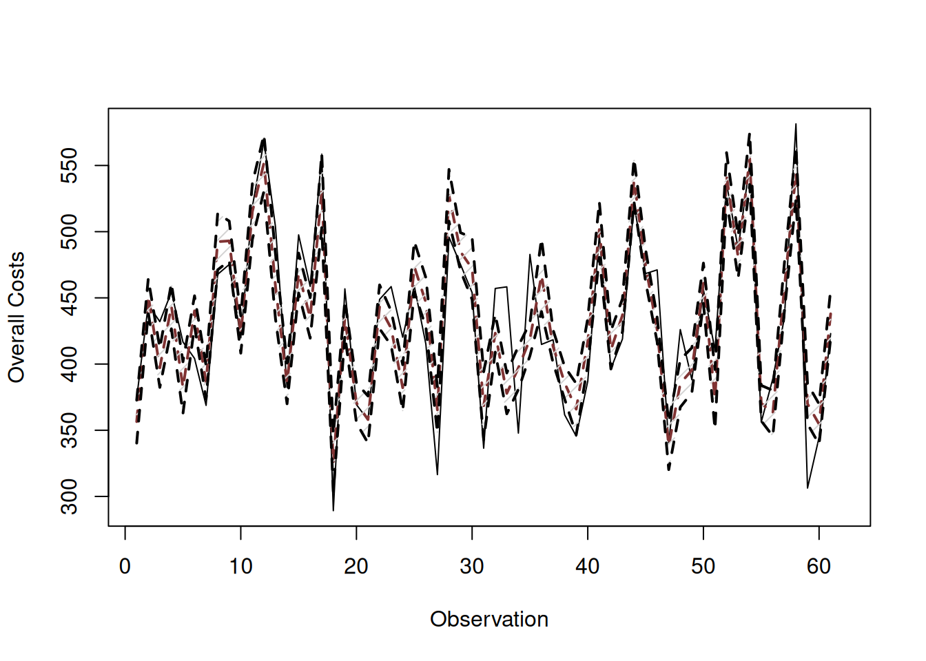
Figure 12.4: Fitted values and confidence interval for the costs model.
It is hard to read this graph because the interval is narrow, and the actual values in it do not help in reading it. But if we zoom in to a specific observation, it would be more readable (Figure 12.5):
# Produce the predicted value and the confidence interval
costsModelMLRCIZoom <- predict(costsModelMLR,
                               interval="confidence",
                               newdata=data.frame(materials=200, size=90,
                                                  projects=3, year=2008))
# Plot the material costs vs fitted
plot(200, costsModelMLRCIZoom$mean,
     xlab="Material costs", ylab="Overall costs",
     ylim=c(costsModelMLRCIZoom$lower, costsModelMLRCIZoom$upper),
     pch=16)
# Add confidence interval
abline(h=c(costsModelMLRCIZoom$lower,
           costsModelMLRCIZoom$upper),
       col=4, lwd=2, lty=2)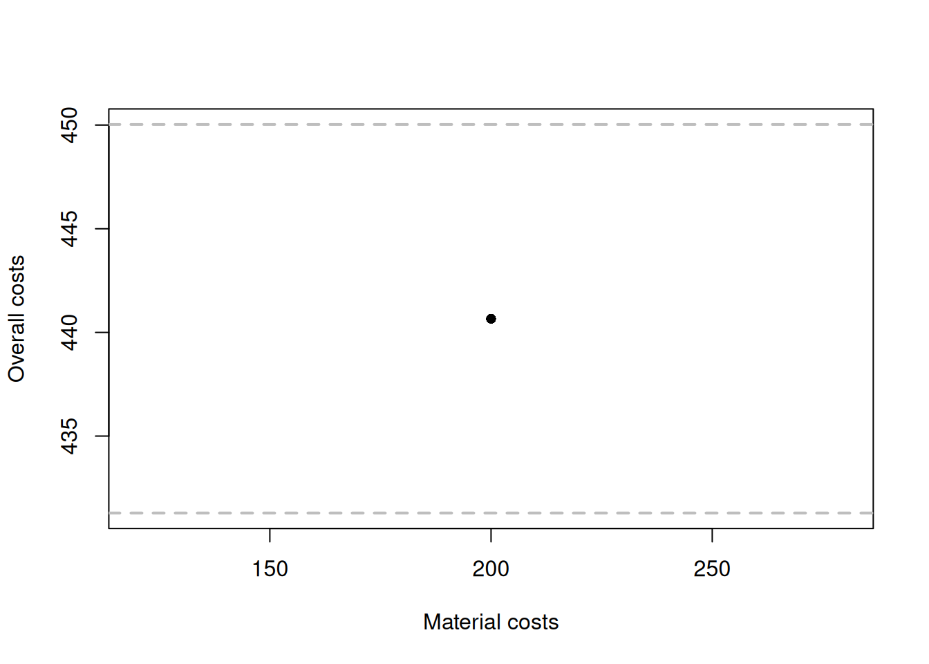
Figure 12.5: Fitted values and confidence interval for the costs model.
What the image in Figure 12.5 shows is that according to the estimated regression, for the project where the material costs were £200k, size of the property was 90 m\(^2\), the crew did 3 projects and the new project was done in the year 2008, the expected overall costs would be 583.2608. But given the uncertainty of the estimates of parameters, the true expected costs should lie between 569.9507 and 596.5709 in 95% of the cases if we repeat the confidence interval construction many times.
Another way of visualising the confidence interval is by plotting the actuals vs fitted figure:
plot(fitted(costsModelMLR), actuals(costsModelMLR),
     xlab="Fitted",ylab="Actuals")
abline(a=0, b=1, col=3, lwd=2, lty=2)
lines(sort(fitted(costsModelMLR)),
      costsModelMLRCI$lower[order(fitted(costsModelMLR))],
      col=4, lwd=2, lty=2)
lines(sort(fitted(costsModelMLR)),
      costsModelMLRCI$upper[order(fitted(costsModelMLR))],
      col=4, lwd=2, lty=2)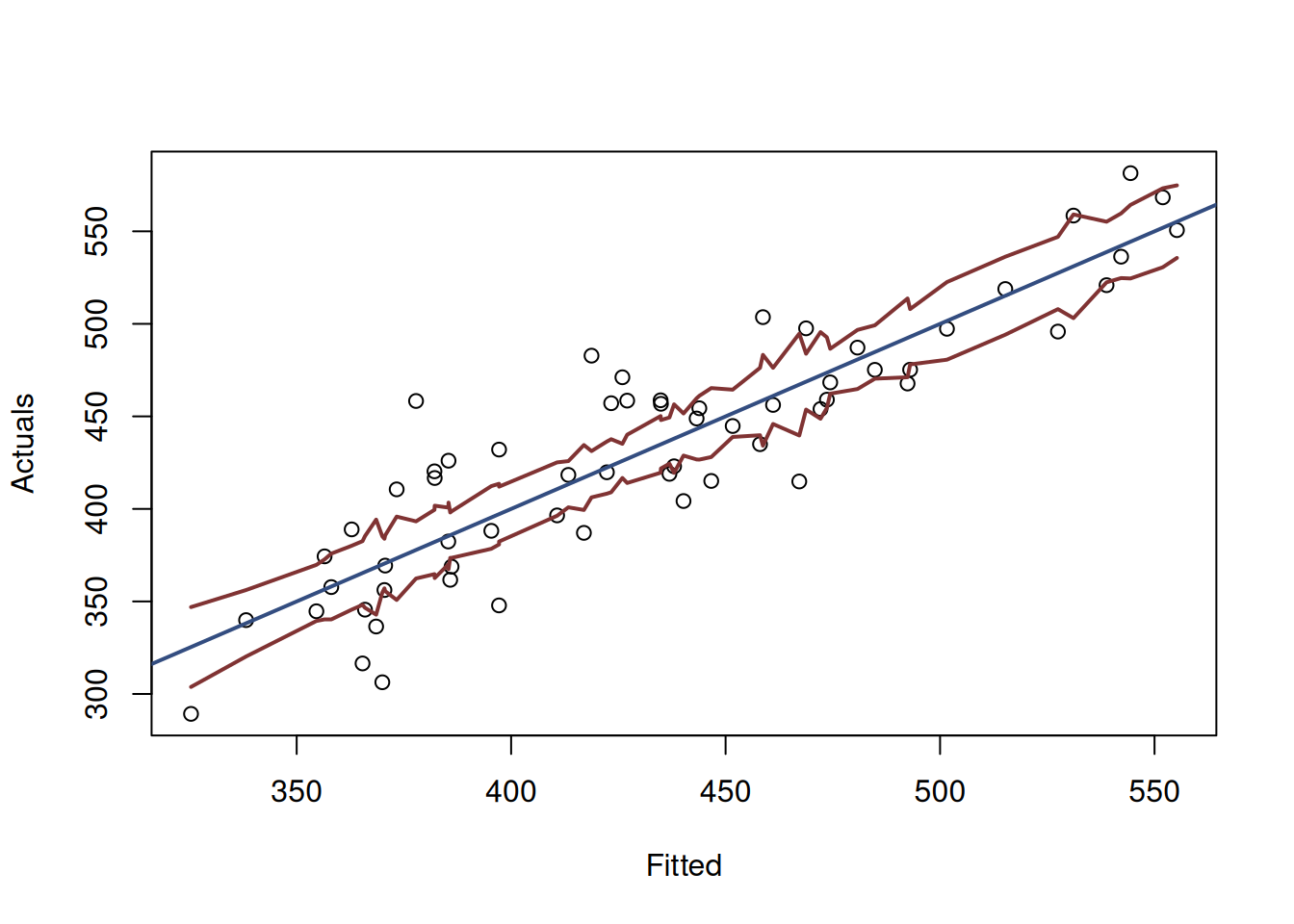
Figure 12.6: Actuals vs Fitted and confidence interval for the costs model.
Figure 12.6 demonstrates the actuals vs fitted plot, together with the 95% confidence interval around the line, demonstrating where the true line would be expected to be in 95% of the cases if we re-estimate the model many times on different samples. We also see that the uncertainty of the regression line is lower in the middle of the data than in the tails. Conceptually, this happens because the regression line, estimated via OLS, always passes through the average point of the data \((\bar{x},\bar{y})\) and the variability in this point is lower than the variability in the tails.
12.3.2 Prediction interval
In case of prediction interval, we are interested in understanding where the actual values lie, not the expected one. For our example, that would mean that we want to know the span of overall costs in the x% of the cases (e.g. 95%) for a project constructed in 2008 that has material costs of £200k, size of the property of 90 squared meters, done by the crew that did 3 projects before it.
The construction of the interval relies on the formula, which is very similar to the one used for the confidence interval: \[\begin{equation} y_j \in (\hat{y}_j + z_{\alpha/2} s_y^2, \hat{y}_j + z_{1-\alpha/2} s_y^2), \tag{12.15} \end{equation}\] where \(s_y^2\) is the standard deviation of the actual values, conditional on the values of the explanatory variables. Its derivation is shown in Subsection 12.3.3. The main difference with the confidence interval is that we now need to rely on the assumption about the distribution of the error term in the model.
Remark. In the formula above, the important assumption is that the error term follows the Normal distribution. We can no longer rely on the CLT, because it only applies to the estimates of parameters. If we cannot assume that the error term follows the Normal distribution, we would need to use either a different one, or to construct the interval using some non-parametric methods.
In R, the interval construction can be done via the very same predict() function with interval="prediction":
Based on this, we can produce an images similar to 12.4 and 12.6.
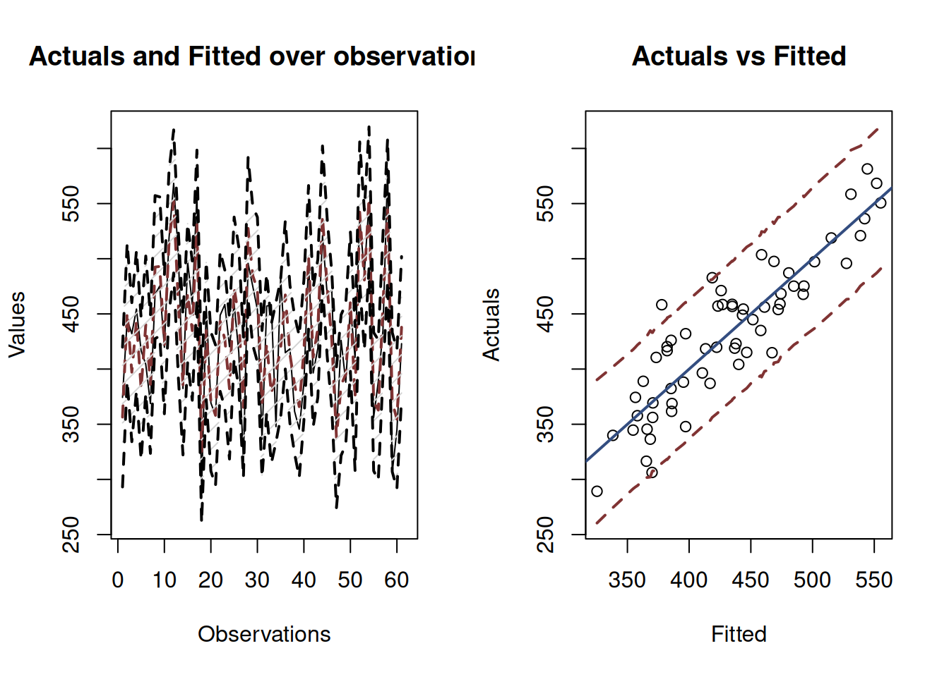
Figure 12.7: Fitted values and prediction interval for the stopping distance model.
Figure 12.7 shows the prediction interval for values over observations and for actuals vs fitted. While the first image is hard to read, we can see that the prediction interval is wider than the confidence one. The second image is more informative, showing that there are some points lying outside of the 95% prediction interval (there are 3 observations outside it). The statistical principles guarantee that asymptotically, if we increase the sample size and repeat the experiment many times, we would have 95% of observations lying inside the interval if the regression assumptions hold.
In forecasting, prediction interval has a bigger importance than the confidence interval. This is because we are typically interested in capturing the uncertainty about the observations, not about the estimate of a line. Typically, the prediction interval would be constructed for some holdout data, which we did not have at the model estimation phase. In the example with costs, we could see what the prediction interval would be in the setting we discussed earlier (materials=200, size=90, projects=3 and year=2008):
costsModelMLRForecast <- predict(costsModelMLR,
                                 newdata=data.frame(materials=200, size=90,
                                                    projects=3, year=2008),
                                 interval="prediction")
plot(costsModelMLRForecast)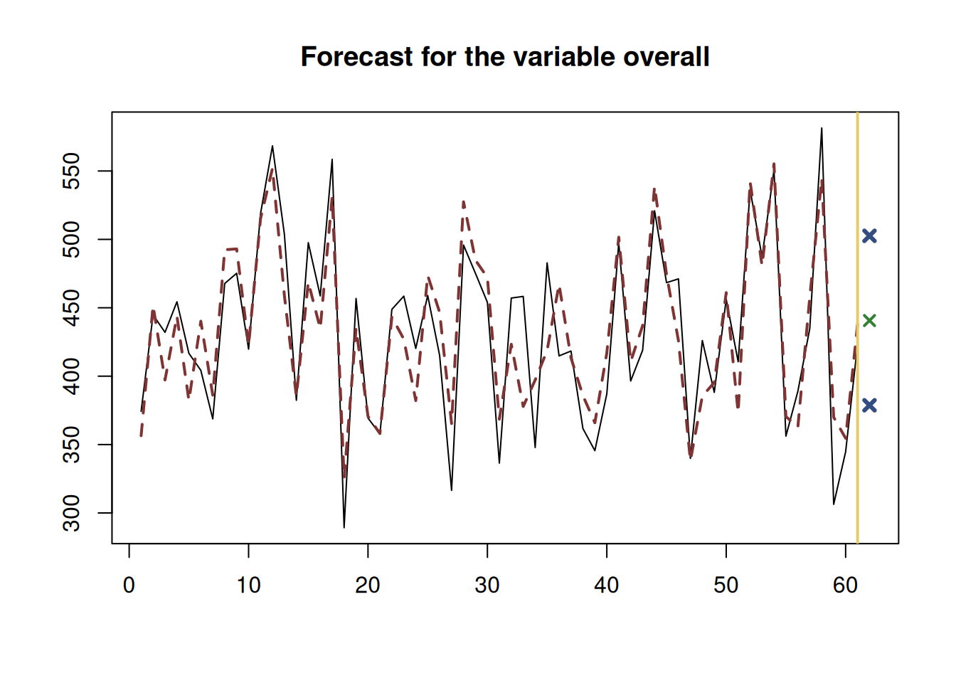
Figure 12.8: Forecast of the overall costs given the material costs of 200, size of 90 squared meters, 3 projects and year 2008.
Figure 12.8 shows the point forecast (the expected overall costs of a project given the values of explanatory variables) and the 95% prediction interval (we expect that in 95% of the cases, the overall costs would be between 495.2759 and 671.2457 thousands of pounds.
12.3.3 Derivations of the variance in regression
The uncertainty of the regression line builds upon the uncertainty of parameters and can be measured via the conditional variance using the formula: \[\begin{equation*} \mathrm{V}(\hat{y}_j| \mathbf{x}_j) = \mathrm{V}(b_0 + b_1 x_{1,j} + b_2 x_{2,j} + \dots + b_{k-1} x_{k-1,j}) , \tag{12.16} \end{equation*}\] which after some simplifications leads to: \[\begin{equation} \mathrm{V}(\hat{y}_j| \mathbf{x}_j) = \sum_{l=0}^{k-1} \mathrm{V}(b_j) x^2_{l,j} + 2 \sum_{l=1}^{k-1} \sum_{i=0}^{l-1} \mathrm{cov}(b_i,b_l) x_{i,j} x_{l,j} , \tag{12.17} \end{equation}\] where \(x_{0,j}=1\). Alternatively, this can be calculated using the compact form of the multiple regression model (11.6): \[\begin{equation*} y_j = \mathbf{x}'_j \boldsymbol{\beta} + \epsilon_j . \end{equation*}\] the fitted values for which are: \[\begin{equation*} \hat{y_j} = \mathbf{x}'_j \boldsymbol{\beta} . \end{equation*}\] Taking the variance of the fitted in that form would involve the covariance matrix of parameters from Section 12.1: \[\begin{equation*} \mathrm{V}(\hat{y_j}| \mathbf{x}_j) = \mathbf{x}'_j \mathrm{V}({\boldsymbol{b}}) \mathbf{x}_j. \end{equation*}\] In any case, we see that the variance of the regression line relies on the variances and covariances of parameters. It can then be used in the construction of the confidence interval for the regression line.
Given that each estimate of parameter \(b_i\) should follow the Normal distribution with a fixed mean and variance due to CLT (Section 6.3), the predicted value \(\hat{y}_j\) will follow it as well. This is because the multiplication of the Normal distribution by a number (the value of an explanatory variable) gives the Normal distribution as well, and the addition of Normal distributions produces another one, but with different parameters. So, we can say that: \[\begin{equation*} \mu_j \sim \mathcal{N}(\hat{y}_j, \mathrm{V}(\hat{y}_j| \mathbf{x}_j)) . \end{equation*}\] We used this property to derive the formula for the confidence interval around the line.
If we are interested in capturing the uncertainty of the actual values, we can refer to prediction interval. In this case we rely on the Normality assumption for the actual values themselves: \[\begin{equation*} y_j = (\hat{y}_j + \epsilon_j) \sim \mathcal{N}(\hat{y}_j, s_y^2) , \end{equation*}\] because we assume that \(\epsilon_j \sim \mathcal{N}(0, {\sigma}^2)\), where \({\sigma}^2\) is the variance of the error term and \(s_y^2 = \mathrm{V}(y_j| \mathbf{x}_j) = \mathrm{V}(\hat{y}_j| \mathbf{x}_j) + \hat{\sigma}^2\) is the estimated of the variance of the response variable conditional on the values of the explanatory variables. The latter can be calculated as: \[\begin{equation} \mathrm{V}(y_j| \mathbf{x}_j) = \mathrm{V}(b_0 + b_1 x_{1,j} + b_2 x_{2,j} + \dots + b_{k-1} x_{k-1,j} + e_j) , \tag{12.18} \end{equation}\] which can be simplified to (if assumptions of regression model hold, see Chapter 15): \[\begin{equation} \mathrm{V}(y_j| \mathbf{x}_j) = \mathrm{V}(\hat{y}_j | \mathbf{x}_j) + \hat{\sigma}^2, \tag{12.19} \end{equation}\] where the variance \(\mathrm{V}(\hat{y}_j | \mathbf{x}_j)\) was calculated above for the confidence interval in formula (12.17). Given that the variance (12.19) is larger than the variance (12.17), the prediction interval will always be wider than the confidence one.