This book is in Open Review. I want your feedback to make the book better for you and other readers. To add your annotation, select some text and then click the on the pop-up menu. To see the annotations of others, click the button in the upper right hand corner of the page

10.1 Ordinary Least Squares (OLS)

For obvious reasons, we do not have the values of parameters from the population: it would be simply impossible to measure heights, diameters and volumes of all eysting trees in the world. This means that we will never know what the true intercept and slope are. But we can get some estimates of these parameters based on the sample of data we have. There are different ways of doing that, and the most popular one is called “Ordinary Least Squares” method. This is the method that was used in the estimation of the model in Figure 10.3. So, how does it work?

Having the sample of data, we can draw a line through the cloud of points and then change the parameters for the intercept and slope until we are satisfied with how the line looks like. This would not be a reliable approach, but what we would be doing in this case is probably just making sure that the line goes somehow in the middle of data. To make this more rigorous, we could use the following simple method:

Remark. This is not how OLS works, but this gives an idea what it implies.

1. Sort all values in ascending order;
2. Split the sample in two halves based on the middle of the explanatory variable (in our case that would be height=76);
3. Calculate mean height and volume in the first half of the data;
4. Calculate mean height and volume of the second half;
5. Draw the line through the points on the plane.

The resulting line is shown in Figure 10.4

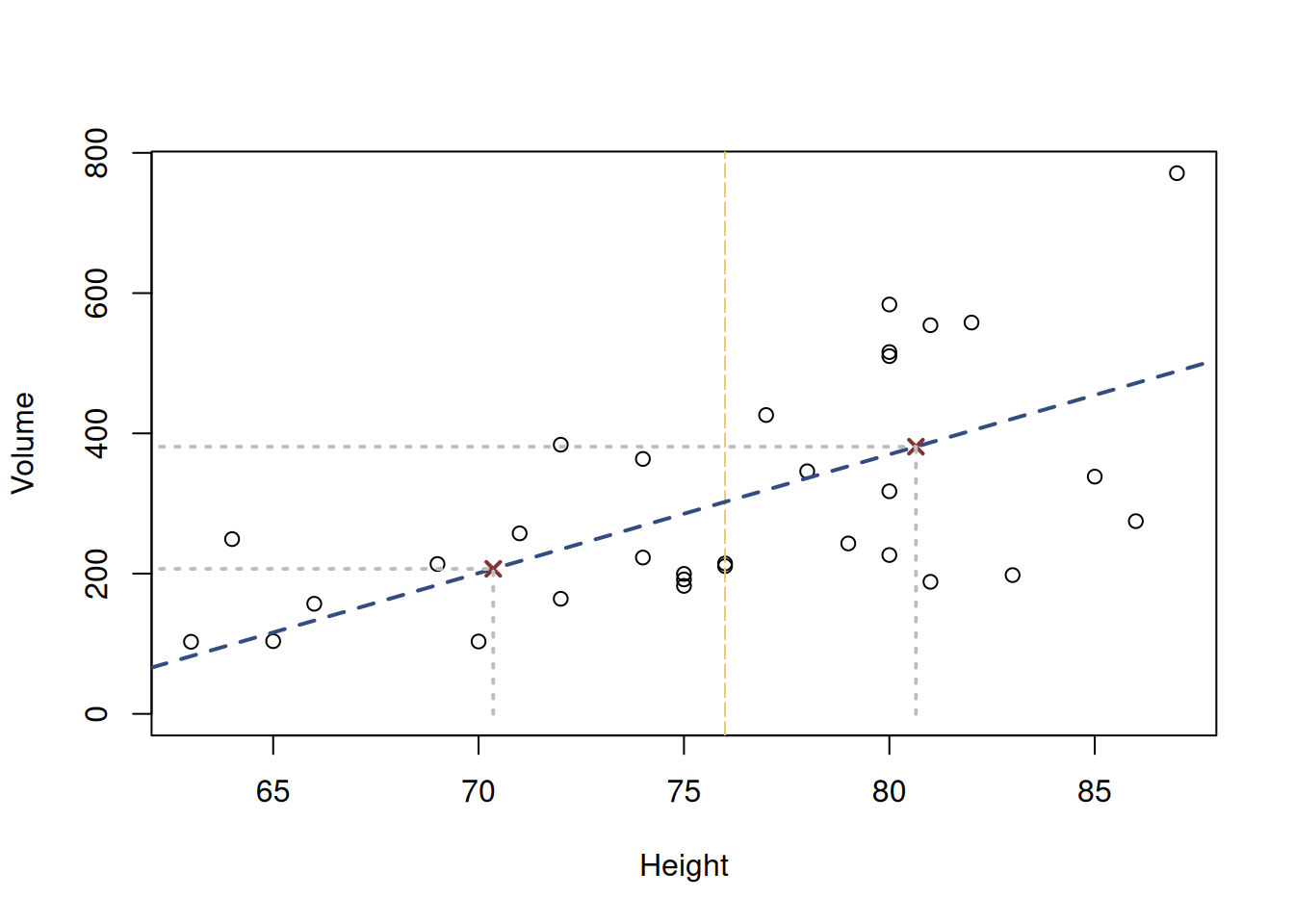
Figure 10.4: Scatterplot diagram between height and volume and the line drawn through two middle points of the data.

The line in the figure represents the average change of volume with the increase of height of trunks. The red crosses show the middle points, the vertical line in the middle shows where the sample is split into two halves. We could improve this method by splitting each half into two halves again, and calculating points for them, or even further splitting each resulting half in halves etc. This method might not be reasonable for the specific sample, but if we had the population data, eventually we would be able to get a collection of points, each one of them representing the mean volume of trees given specific height.

But there is an easier way to do something similar but more practical. We could draw an arbitrary line, picking some estimates of parameters $b_0$ and $b_1$.

Remark. We never know the true values of $\beta_0$ and $\beta_1$, which is why when we estimate a model, we should substitute them with $b_0$ and $b_1$. This way we show that we deal with just some estimates of the true parameters.

After that we can calculate errors for each of observations, as we did before, but this time, because we do not know the true line, and we are only trying to get the best possible estimates of parameters, we should denote each error as $e_j$ instead of $\epsilon_j$, which in general they can be calculated as $e_j = y_j - \hat{y}_j$, where $\hat{y}_j$ is the value of the regression line (aka “fitted” value) for each specific value of explanatory variable.

For example, for the height of tree of 64 meters, the actual volume is 249.2, while the fitted value would be 117.052. The resulting error (or residual of model) is 249.2 - 117.052 = 132.148. We could collect all these errors of the model for all available trees based on their heights and this would result in a vector of positive and negative values like this:

##           1           2           3           4           5           6 
## -106.477610  -28.789597    1.185608  -76.452815 -191.191239 -212.466444 
##           7           8           9          10          11          12 
##    9.072800 -104.365623 -137.553636  -87.265623 -105.616034  -91.603226 
##          13          14          15          16          17          18 
##  -87.803226   19.459993  -95.165623  -48.528021 -102.941649 -181.879252 
##          19          20          21          22          23          24 
##   32.284787  132.148006   12.721569  -46.653636   92.071979  143.247185 
##          25          26          27          28          29          30 
##  108.359172  174.708761  163.071158  219.646364  151.846364  146.046364 
##          31 
##  298.883145

These residuals are obtained from the following mathematical formula, given some values of $b_0$ and $b_1$: $$\begin{equation} e_j = y_j - {b}_0 - {b}_1 x_j. \tag{10.3} \end{equation}$$ If we needed to estimate parameters ${b}_0$ and ${b}_1$ of the model, we would want to minimise those distances by changing the parameters of the model. This would correspond to drawing a line going through the middle of the series, in a way connecting all the possible mean points in the data. Visually this is shown in Figure 10.5, where the line somehow goes through the data, and we calculate errors from it.

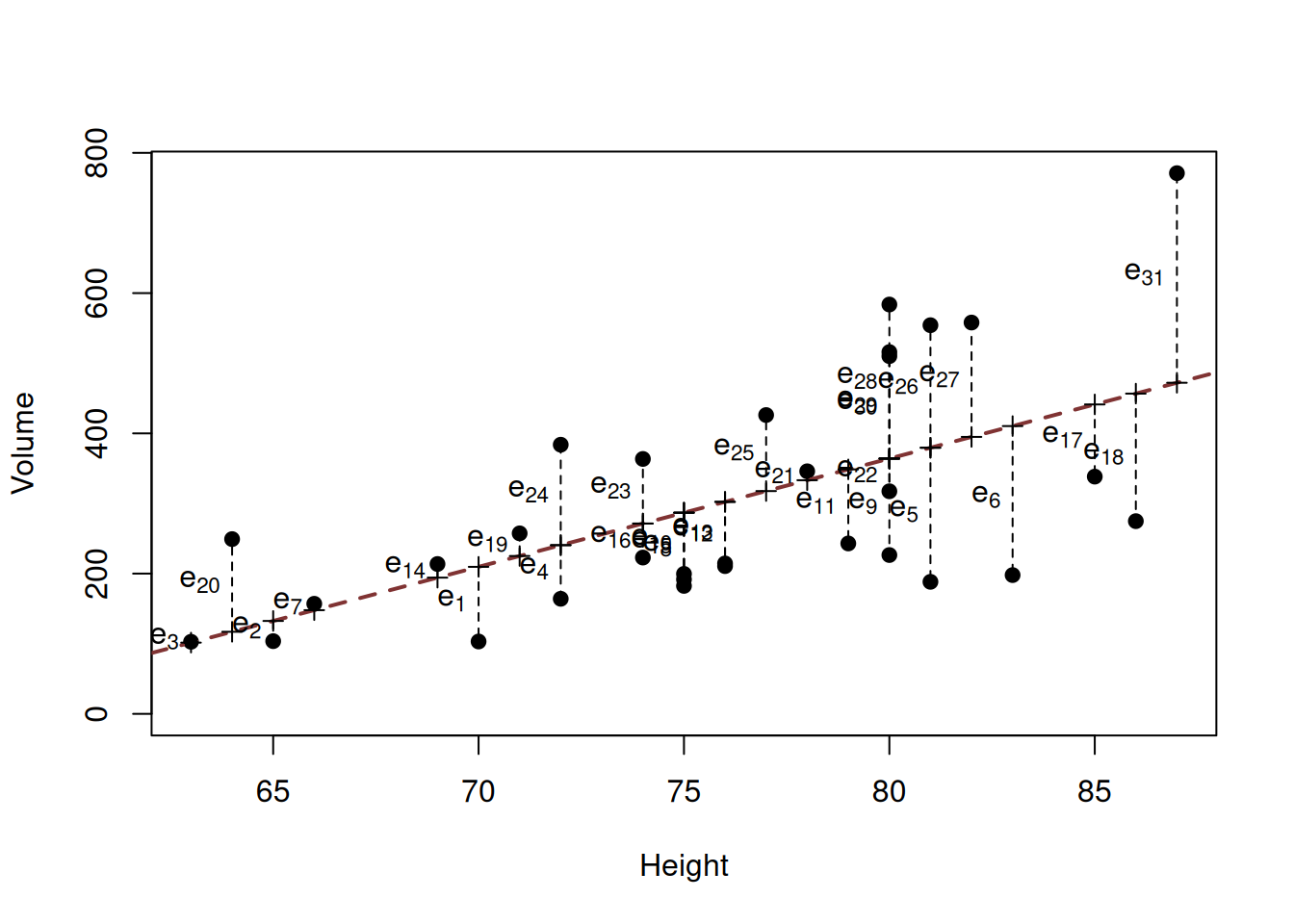
Figure 10.5: Scatterplot diagram between height and volume and the OLS line.

The problem is that some errors are positive, while the others are negative (see the middle image in Figure 10.6). If we just sum them up, they will cancel each other out, and we would loose the information about the distance. The simplest way to get rid of sign and keep the distance is by taking squares of each error, as shown in the bottom image in Figure 10.6.

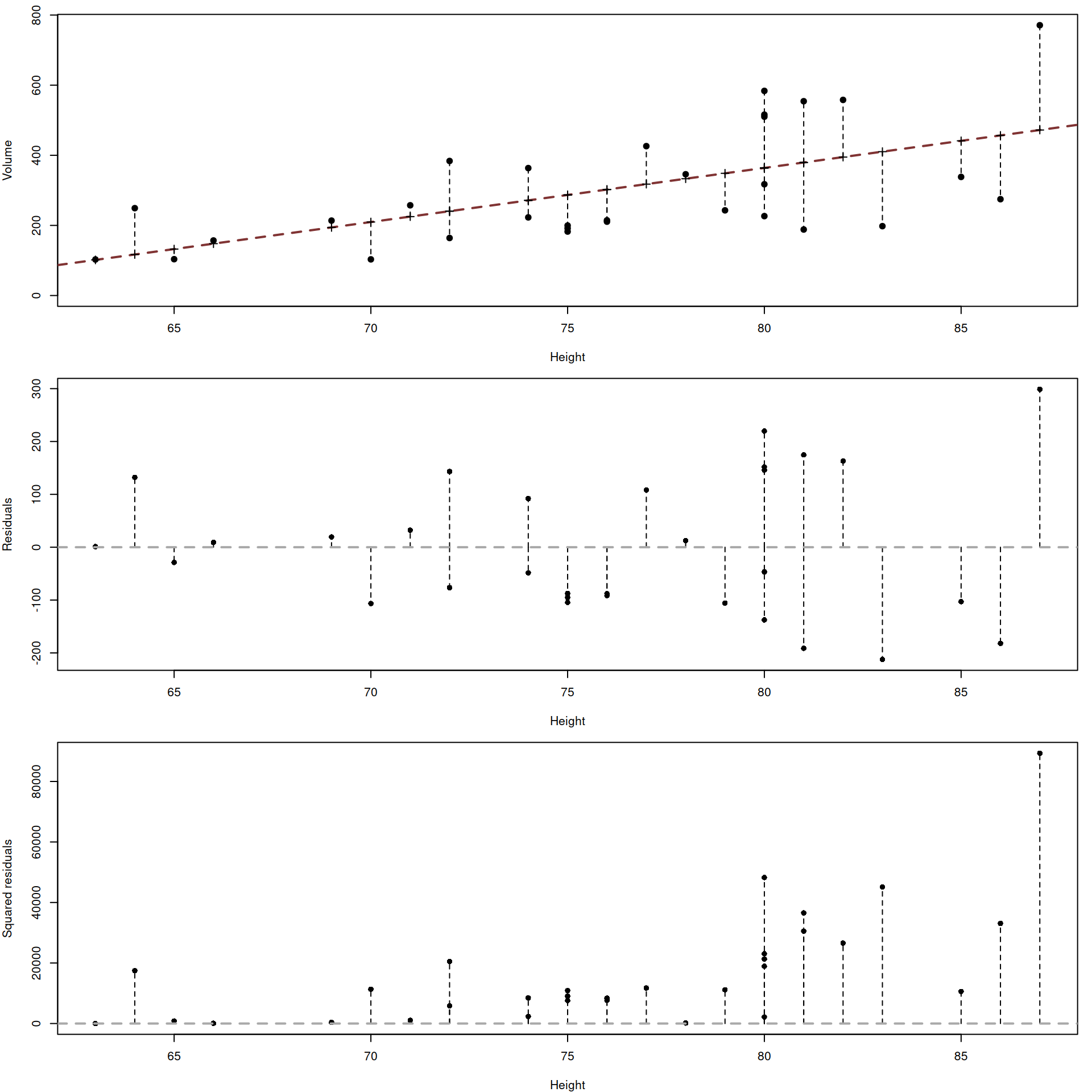
Figure 10.6: Volume, residuals and their squared values plotted agains the height of trees.

If we then sum up all the squared residuals, we will end up with something called “Sum of Squared Errors”: $$\begin{equation} \mathrm{SSE} = \sum_{j=1}^n e_j^2 . \tag{10.4} \end{equation}$$ If we now minimise SSE by changing values of parameters ${b}_0$ and ${b}_1$, we will find the parameters that would guarantee that the line goes through the cloud of points. Luckily, we do not need to use any fancy optimisers for this, as there is an analytical solution to this: $$\begin{equation} \begin{aligned} {b}_1 = & \frac{\mathrm{cov}(x,y)}{\mathrm{V}(x)} \\ {b}_0 = & \bar{y} - {b}_1 \bar{x} \end{aligned} , \tag{10.5} \end{equation}$$ where $\bar{x}$ is the mean of the explanatory variable $x_j$ (height in our example) and $\bar{y}$ is the mean of the response variables $y_j$ (volume).

Proof. In order to get (10.5), we should first insert (10.3) in (10.4) to get: $$\begin{equation*} \mathrm{SSE} = \sum_{j=1}^n (y_j - {b}_0 - {b}_1 x_j)^2 . \end{equation*}$$ This can be expanded to: $$\begin{equation*} \begin{aligned} \mathrm{SSE} = & \sum_{j=1}^n y_j^2 - 2 b_0 \sum_{j=1}^n y_j - 2 b_1 \sum_{j=1}^n y_j x_j + \\ & n b_0^2 + 2 b_0 b_1 \sum_{j=1}^n x_j + b_1^2 \sum_{j=1}^n x_j^2 \end{aligned} \end{equation*}$$ Given that we need to find the values of parameters $b_0$ and $b_1$ minimising SSE, we can take a derivative of SSE with respect to $b_0$ and $b_1$, equating them to zero to get the following System of Normal Equations: $$\begin{equation*} \begin{aligned} & \frac{d \mathrm{SSE}}{d b_0} = -2 \sum_{j=1}^n y_j + 2 n b_0 + 2 b_1 \sum_{j=1}^n x_j = 0 \\ & \frac{d \mathrm{SSE}}{d b_1} = -2 \sum_{j=1}^n y_j x_j + 2 b_0 \sum_{j=1}^n x_j + 2 b_1 \sum_{j=1}^n x_j^2 = 0 \end{aligned} \end{equation*}$$

Solving this system of equations for $b_0$ and $b_1$ we get: $$\begin{equation} \begin{aligned} & b_0 = \frac{1}{n}\sum_{j=1}^n y_j - b_1 \frac{1}{n}\sum_{j=1}^n x_j \\ & b_1 = \frac{n \sum_{j=1}^n y_j x_j - \sum_{j=1}^n y_j \sum_{j=1}^n x_j}{n \sum_{j=1}^n x_j^2 - \left(\sum_{j=1}^n x_j \right)^2} \end{aligned} \tag{10.6} \end{equation}$$ In the system of equations (10.6), we have the following elements:

1. $\bar{y}=\frac{1}{n}\sum_{j=1}^n y_j$,
2. $\bar{x}=\frac{1}{n}\sum_{j=1}^n x_j$,
3. $\mathrm{cov}(x,y) = \frac{1}{n}\sum_{j=1}^n y_j x_j - \frac{1}{n^2}\sum_{j=1}^n y_j \sum_{j=1}^n x_j$,
4. $\mathrm{V}(x) = \frac{1}{n}\sum_{j=1}^n x_j^2 - \left(\frac{1}{n} \sum_{j=1}^n x_j \right)^2$,

which after inserting in (10.6) lead to (10.5).

Remark. If for some reason ${b}_1=0$ in (10.5) (for example, because the covariance between $x$ and $y$ is zero, implying that they are not correlated), then the intercept ${b}_0 = \bar{y}$, meaning that the global average of the data would be the best predictor of the variable $y_j$.

This method of estimation of parameters based on the minimisation of SSE, is called “Ordinary Least Squares”, because by using this method we get the least possible squares of errors for the data. The word “ordinary” means that this is one of the basic estimation techniques. There are other least squares techniques, which we are not yet discussing in this book. The method is simple and does not require any specific assumptions: we just minimise the overall distance between the line and the points by changing the values of parameters.

Example 10.2 For the problem with trees, we can use the lm() function from the stats package in R to get the OLS estimates of parameters. This is done in the following way:

slmTrees <- lm(volume~height, SBA_Chapter_10_Trees)
slmTrees

## 
## Call:
## lm(formula = volume ~ height, data = SBA_Chapter_10_Trees)
## 
## Coefficients:
## (Intercept)       height  
##     -870.95        15.44

The syntax of the function implies that we use volume as the response variable and height as the explanatory one. The resulting model in our notations has $b_0=$ -870.95 and $b_1=$ 15.44, its equation can be written as: $volume_j=$ -870.95 $+$ 15.44 $height_j+e_j$.

While we can make some conclusions based on the simple linear regression, we know that in real life we rarely see bivariate relations - typically a variable is influenced by a set of variables, not just by one. This implies that the correct model would typically include many explanatory variables. This is why we only discuss the simple linear regression for educational purpose and generally, do not recommend to use it in real life situations.