2.6 Bayes’ theorem
One of the common problems we have faced at some point of our online lives is the problem of detecting spam. Consider a situation motivated by the real life scenario, where we track the words in the received emails and depending on some of them, we can assign probability of the email being or not being spam. If this probability is higher than some pre-specified threshold, we can then filter out the message and do efficient spam detection. This is in essence what many mail agents do under the hood, although our case is a crude simplification.
But before we even look at the new email, we have some existing information based on the general flow of emails. This is our initial, or “prior” belief about the probability of an email being spam. We assume the following for this example:
- The probability that any given email is spam: P(Spam) = 0.4 (or 40%)
- The probability that any given email is not spam: P(Not Spam) = 0.6 (or 60%)
We assume that this is the case for our toy example, although in real life these can differ substantially. Next, we have information derived from a large set of training data. This data tells us how frequently the word “discount” appears in emails that are known to be spam versus those that are not. These are our conditional probabilities:
- The probability of seeing the word “discount” given the email is spam: P(“discount”|Spam) = 0.7 (or 70%)
- The probability of seeing the word “discount” given the email is not spam: P(“discount”|Not Spam) = 0.1 (or 10%)
Now, the main question of interest for us is to understand what is the probability that an email is spam if the word ‘discount’ appears in it. i.e. we need to find P(Spam | “discount”).
But how can we do that?
First, we plot the tree diagram to better understand what we have and what we are missing. Here are the notations we use in that figure:
- “Spam” event is denoted with “S”,
- “Not Spam” is “NS”,
- The word “discount” is in the text - “D”,
- The word “discount” is not in the text - “ND”.
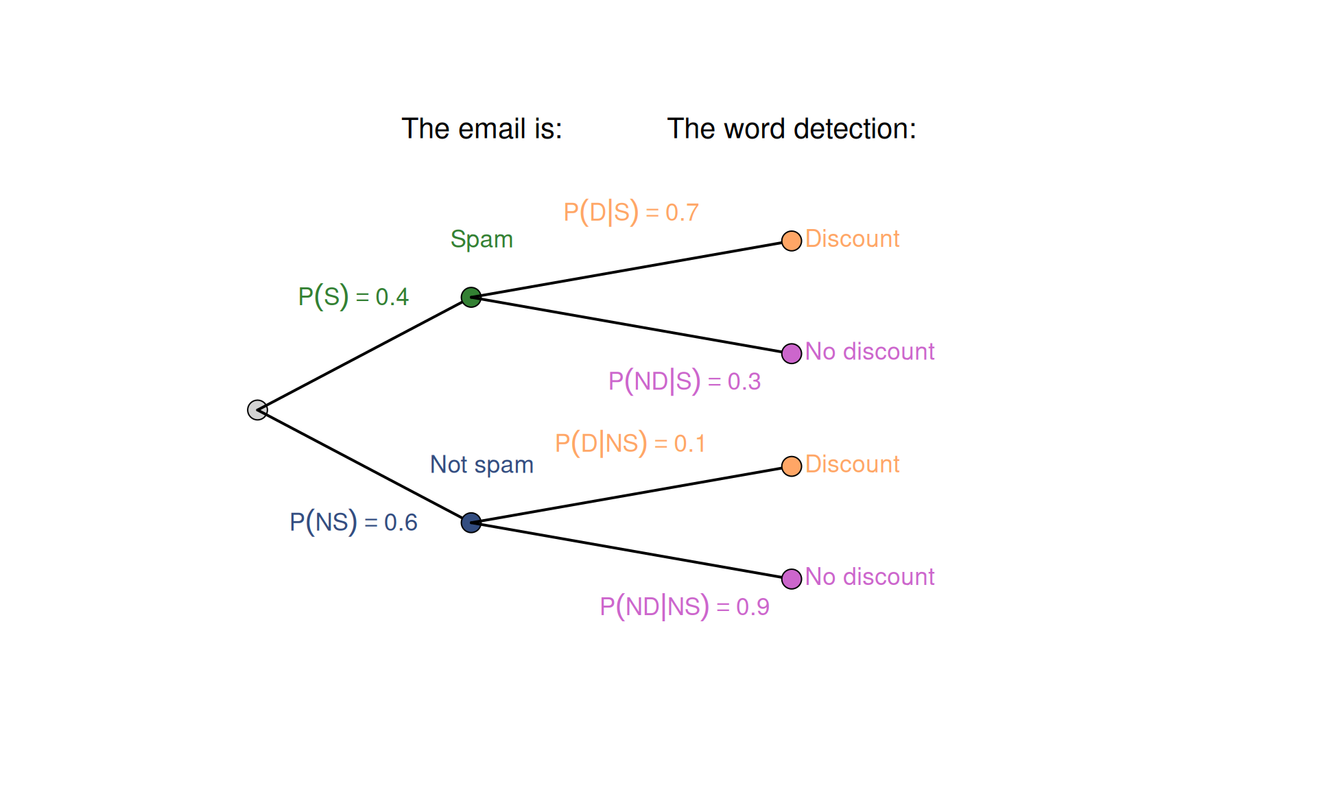
Figure 2.6: Tree diagram for the spam detection example.
As we see in the Tree diagram in Figure 2.6, we know all the probabilities for all the outcomes. So, what is the problem then? The problem is that we need to invert it to get the answer to our question, i.e. build a new tree where the word “discount” is the first vertex (Figure 2.7).
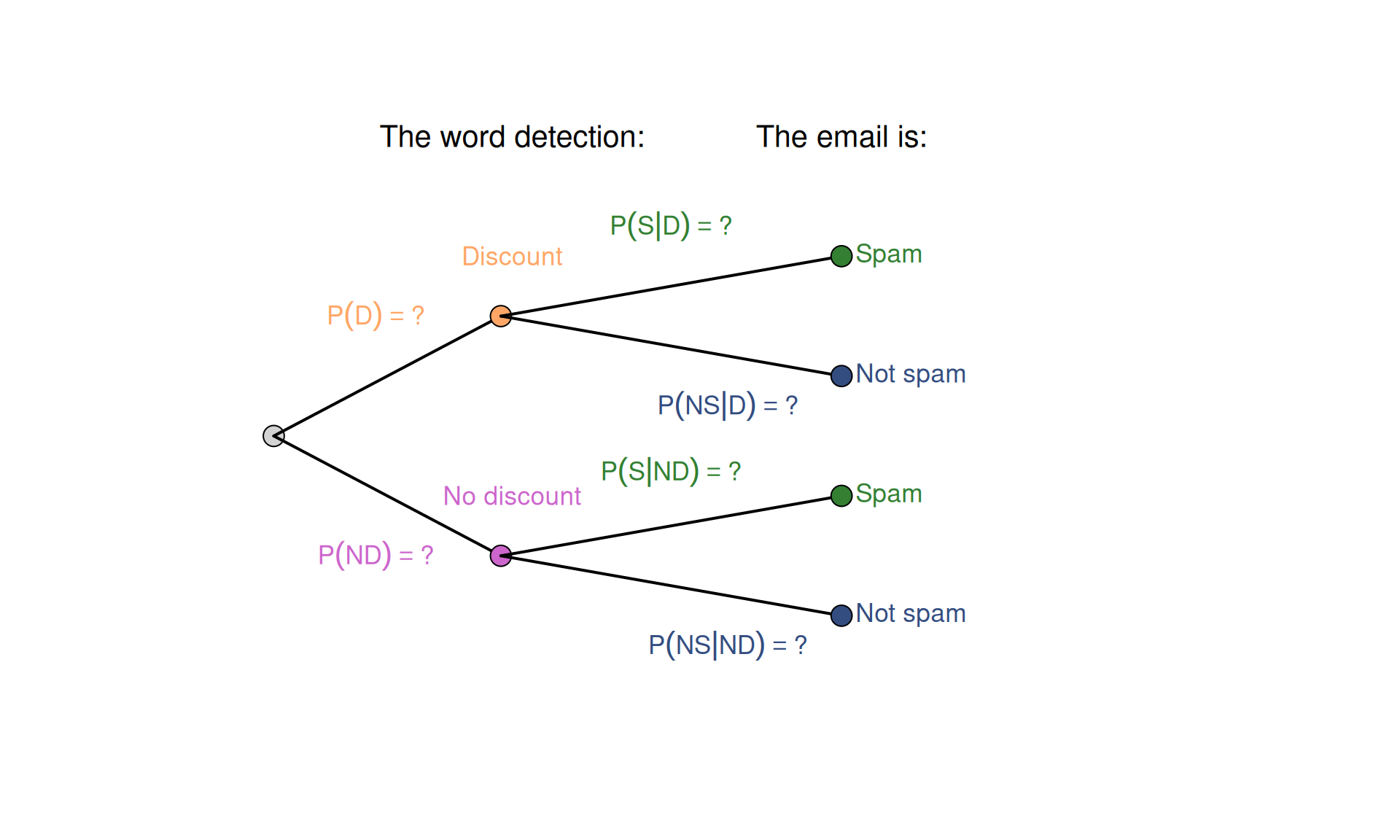
Figure 2.7: Tree diagram for the spam detection example, starting from the word ‘discount’.
In the tree diagram in Figure 2.7, we can easily get the probabilities of having and not having the word “discount”. This can be done using the Law of Total Probability (Section 2.5): \[\begin{equation*} P(D) = P(D|S) P(S) + P(D|NS) P(NS) = 0.7 \times 0.4 + 0.1 \times 0.6 = 0.34 . \end{equation*}\] Given that having and not having the word “discount” are two mutually exclusive events, \(P(ND) = 1 - P(D) = 0.66\). Although this helps, we still do not know how to get to the answer of our question.
So, we should take a step back to the multiplication law from Section 2.4. We can notice that in the example we had, we can work out the final probability equally in any sequence: if we first have event B and then event A, or if we we have first A and then B. In our example with vampires, the order did not matter (the first student becomes first no matter what). But in general, this means that the probability of this joint outcome can be calculated in one of two possible ways: \[\begin{equation} P(A \cap B) = P(B) \times P(A|B) = P(A) \times P(B|A) . \tag{2.9} \end{equation}\]
For the example at hand, this can be written as: \[\begin{equation*} P(S \cap D) = P(D) \times P(S|D) = P(S) \times P(D|S) , \end{equation*}\] which means that the probability of the email containing the word “discount” and being spam given that it contains that word is the same as the probability of the email being spam and containing the word “discount” given that it is spam. This is useful because we can use this equality for our calculations to get the inverse probability we need by regrouping the elements in the equation to:
\[\begin{equation} P(S|D) = \frac{P(S) \times P(D|S)}{P(D)} . \tag{2.10} \end{equation}\] Equation (2.10) is called the Bayes’ equation and allows getting the “posterior” probability (\(P(S|D)\)) given the prior (\(P(S)\)) and some new information (\(P(D|S)\) and \(P(D)\)).
In our case, we have all the probabilities to insert in (2.10):
- \(P(S) = 0.4\);
- \(P(D|S) = 0.7\);
- \(P(D) = 0.34\) - calculated earlier.
Inserting them in the formula (2.10) gives us the answer: \[\begin{equation*} P(S|D) = \frac{0.4 \times 0.7}{0.34} \approx 0.82 . \tag{2.10} \end{equation*}\]
This resulting probability tells us that there is approximately an 82% chance that the email is spam if it contains the word “discount”. Notice how observing this single word has allowed us to update our belief. We started with a prior probability of 40% and, after considering the evidence, have arrived at a revised (“posterior”) probability of 82%. If we set the threshold for filtering the emails as spam, for example, to 80%, any email that would contain the word “discount” would be flagged as one. In reality, the detection systems would rely on sequences of words (tokens) instead of just one word, and the specific probabilities would differ from the ones we used above. But the main principles of the Bayes’ theorem would hold.
2.6.1 Mathematical derivation
The theorem’s origins trace back to the work of the Reverend Thomas Bayes, whose work “An Essay Toward Solving a Problem in the Doctrine of Chances” was published posthumously in 1764 (Bayes?). The derivation begins with the multiplication law for two events, A and B, which states that the probability of both events occurring together can be expressed in two ways (as we saw in equation (2.9)): \[\begin{equation*} P(A \cap B) = P(B) \times P(A|B) = P(A) \times P(B|A) . \end{equation*}\] From this equality, we can isolate P(A|B) through simple algebraic rearrangement to arrive to the fundamental form of Bayes’ theorem: \[\begin{equation} P(A|B) = \frac{P(A) \times P(B|A)}{P(B)} . \tag{2.10} \end{equation}\]
Each component of the theorem has a specific name and plays a distinct role in the process of updating our beliefs. This structure is what makes the theorem so powerful for statistical inference.
- Posterior Probability \(P(A | B)\);
- Conditional Probability \(P(B | A)\);
- Prior Probability \(P(A)\);
- Marginal Probability \(P(B)\).
The probability (3) is the initial probability of event A occurring, based on existing information before the new evidence is considered. The marginal probability \(P(B)\) is the overall probability of observing the new information B. This is often called the evidence or normalising constant. It ensures that the final posterior probabilities sum to 1, by accounting for the overall probability of observing the evidence across all possible hypotheses.