12.2 Hypothesis testing
Another way to look at the uncertainty of parameters is to test a statistical hypothesis. As it was discussed in Section 7, I personally think that hypothesis testing is a less useful instrument for these purposes than the confidence interval and that it might be misleading in some circumstances. Nonetheless, it has its merits and can be helpful if an analyst knows what they are doing. In order to test the hypothesis, we need to follow the procedure, described in Section 7.
12.2.1 Regression parameters
The classical hypotheses for the parameters are formulated in the following way: \[\begin{equation} \begin{aligned} \mathrm{H}_0: \beta_i = 0 \\ \mathrm{H}_1: \beta_i \neq 0 \end{aligned} . \tag{12.3} \end{equation}\] This formulation of hypotheses comes from the idea that we want to check if the effect estimated by the regression is indeed there (i.e. statistically significantly different from zero). Note however, that as in any other hypothesis testing, if you fail to reject the null hypothesis, this only means that you do not know, we do not have enough evidence to conclude anything. This does not mean that there is no effect and that the respective variable can be removed from the model. In case of simple linear regression, the null and alternative hypothesis can be represented graphically as shown in Figure 12.4.
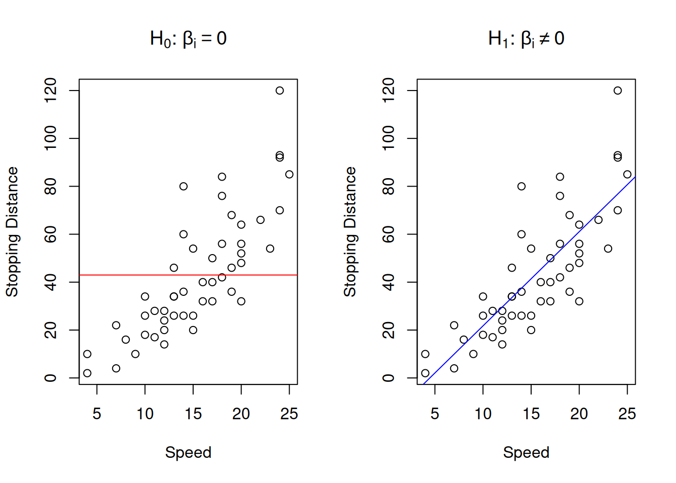
Figure 12.4: Graphical presentation of null and alternative hypothesis in regression context
The graph on the left in Figure 12.4 demonstrates how the true model could look if the null hypothesis was true - it would be just a straight line, parallel to x-axis. The graph on the right demonstrates the alternative situation, when the parameter is not equal to zero. We do not know the true model, and hypothesis testing does not tell us, whether the hypothesis is true or false, but if we have enough evidence to reject H\(_0\), then we might conclude that we see an effect of one variable on another in the data. Note, as discussed in Section 7, the null hypothesis is always wrong, and it will inevitably be rejected with the increase of sample size.
Given the discussion in the previous subsection, we know that the parameters of regression model will follow normal distribution, as long as all assumptions are satisfied (including those for CLT). We also know that because the standard errors of parameters are estimated, we need to use Student’s distribution, which takes the uncertainty about the variance into account. Based on this, we can say that the following statistics will follow t with \(n-k\) degrees of freedom: \[\begin{equation} \frac{b_i - 0}{s_{b_i}} \sim t(n-k) . \tag{12.4} \end{equation}\] After calculating the value and comparing it with the critical t-value on the selected significance level or directly comparing p-value based on (12.4) with the significance level, we can make conclusions about the hypothesis.
The context of regression provides a great example, why we never accept hypothesis and why in the case of “Fail to reject H\(_0\)”, we should not remove a variable (unless we have more fundamental reasons for doing that). Consider an example, where the estimated parameter \(b_1=0.5\), and its standard error is \(s_{b_1}=1\), we estimated a simple linear regression on a sample of 30 observations, and we want to test, whether the parameter in the population is zero (i.e. hypothesis (12.3)) on 1% significance level. Inserting the values in formula (12.4), we get: \[\begin{equation*} \frac{|0.5 - 0|}{1} = 0.5, \end{equation*}\] with the critical value for two-tailed test of \(t_{0.01}(30-2)\approx 2.76\). Comparing t-value with the critical one, we would conclude that we fail to reject H\(_0\) and thus the parameter is not statistically different from zero. But what would happen if we check another hypothesis: \[\begin{equation*} \begin{aligned} \mathrm{H}_0: \beta_1 = 1 \\ \mathrm{H}_1: \beta_1 \neq 1 \end{aligned} . \end{equation*}\] The procedure is the same, the calculated t-value is: \[\begin{equation*} \frac{|0.5 - 1|}{1} = 0.5, \end{equation*}\] which leads to exactly the same conclusion as before: on 1% significance level, we fail to reject the new H\(_0\), so the value is not distinguishable from 1. So, which of the two is correct? The correct answer is “we do not know”. The non-rejection region just tells us that uncertainty about the parameter is so high that it also include the value of interest (0 in case of the classical regression analysis). If we constructed the confidence interval for this problem, we would not have such confusion, as we would conclude that on 1% significance level the true parameter lies in the region \((-2.26, 3.26)\) and can be any of these numbers.
In R, if you want to test the hypothesis for parameters, I would recommend using lm() function for regression:
##
## Call:
## lm(formula = dist ~ speed, data = cars)
##
## Residuals:
##     Min      1Q  Median      3Q     Max
## -29.069  -9.525  -2.272   9.215  43.201
##
## Coefficients:
##             Estimate Std. Error t value Pr(>|t|)
## (Intercept) -17.5791     6.7584  -2.601   0.0123 *
## speed         3.9324     0.4155   9.464 1.49e-12 ***
## ---
## Signif. codes:  0 '***' 0.001 '**' 0.01 '*' 0.05 '.' 0.1 ' ' 1
##
## Residual standard error: 15.38 on 48 degrees of freedom
## Multiple R-squared:  0.6511, Adjusted R-squared:  0.6438
## F-statistic: 89.57 on 1 and 48 DF,  p-value: 1.49e-12
This output tells us that when we consider the parameter for the variable speed, we reject the standard H\(_0\) on the pre-selected 1% significance level (comparing the level with p-value in the last column of the output). Note that we should first select the significance level and only then conduct the test, otherwise we would be bending reality for our needs.
12.2.2 Regression line
Finally, in regression context, we can test another hypothesis, which becomes useful, when a lot of parameters of the model are very close to zero and seem to be insignificant on the selected level: \[\begin{equation} \begin{aligned} \mathrm{H}_0: \beta_1 = \beta_2 = \dots = \beta_{k-1} = 0 \\ \mathrm{H}_1: \beta_1 \neq 0 \vee \beta_2 \neq 0 \vee \dots \vee \beta_{k-1} \neq 0 \end{aligned} , \tag{12.5} \end{equation}\] which translates into normal language as “H\(_0\): all parameters (except for intercept) are equal to zero; H\(_1\): at least one parameter is not equal to zero”. This hypothesis is only needed, when you have a model with many statistically insignificant variables and want to see if the model explains anything. This is done using F-test, which can be calculated based on sums of squares: \[\begin{equation*} F = \frac{ SSR / (k-1)}{SSE / (n-k)} \sim F(k-1, n-k) , \end{equation*}\] where the sums of squares are divided by their degrees of freedom. The test is conducted in the similar manner as any other test (see Section 7): after choosing the significance level, we can either calculate the critical value of F for the specified degrees of freedom, or compare it with the p-value from the test to make a conclusion about the null hypothesis.
This hypothesis is not very useful, when the parameter are significant and coefficient of determination is high. It only becomes useful in difficult situations of poor fit. The test on its own does not tell if the model is adequate or not. And the F value and related p-value is not comparable with respective values of other models. Graphically, this test checks, whether in the true model the slope of the straight line on the plot of actuals vs fitted is different from zero. An example with the same stopping distance model is provided in Figure 12.5.
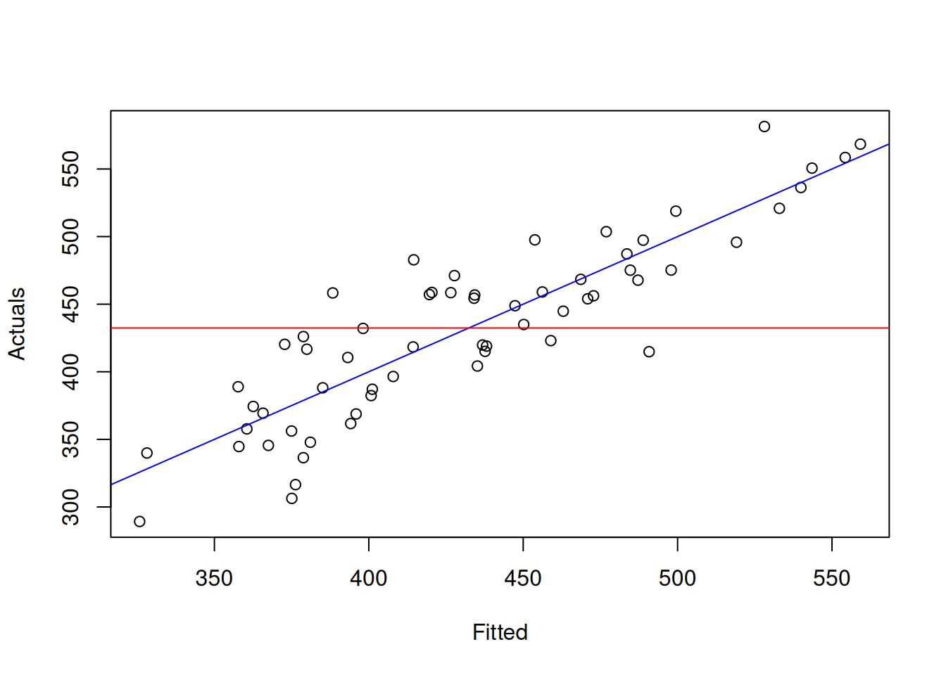
Figure 12.5: Graphical presentation of F test for regression model.
What the test is tries to get insight about, is whether in the true model the blue line coincides with the red line (i.e. the slope is equal to zero, which is only possible, when all parameters are zero). If we have enough evidence to reject the null hypothesis, then this means that the slopes are different on the selected significance level.
Here is an example with the speed model discussed above with the significance level of 1%:
##    value
## 89.56711## [1] 7.194218## value
## 1.489919e-12In the output above, the critical value is lower than the calculated, so we can reject the H\(_0\), which means that there is something in the model that explains the variability in the variable dist. Alternatively, we could focus on p-value. We see that the it is lower than the significance level of 1%, so we reject the H\(_0\) and come to the same conclusion as above.