12.3 Regression line uncertainty
Given the uncertainty of estimates of parameters, the regression line itself and the points around it will be uncertain. This means that in some cases we should not just consider the predicted values of the regression \(\hat{y}_j\), but also the uncertainty around them.
The uncertainty of the regression line builds upon the uncertainty of parameters and can be measured via the conditional variance in the following way: \[\begin{equation} \mathrm{V}(\hat{y}_j| \mathbf{x}_j) = \mathrm{V}(b_0 + b_1 x_{1,j} + b_2 x_{2,j} + \dots + b_{k-1} x_{k-1,j}) , \tag{12.6} \end{equation}\] which after some simplifications leads to: \[\begin{equation} \mathrm{V}(\hat{y}_j| \mathbf{x}_j) = \sum_{l=0}^{k-1} \mathrm{V}(b_j) x^2_{l,j} + 2 \sum_{l=1}^{k-1} \sum_{i=0}^{l-1} \mathrm{cov}(b_i,b_l) x_{i,j} x_{l,j} , \tag{12.7} \end{equation}\] where \(x_{0,j}=1\). As we see, the variance of the regression line involves variances and covariances of parameters. This variance can then be used in the construction of the confidence interval for the regression line. Given that each estimate of parameter \(b_i\) will follow normal distribution with a fixed mean and variance due to CLT, the predicted value \(\hat{y}_j\) will follow normal distribution as well. This can be used in the construction of the confidence interval, in a manner similar to the one discussed in Section 6.4: \[\begin{equation} \mu_j \in (\hat{y}_j + t_{\alpha/2}(n-k) s_{\hat{y}_j}, \hat{y}_j + t_{1-\alpha/2}(n-k) s_{\hat{y}_j}), \tag{12.8} \end{equation}\] where \(s_{\hat{y}_j}=\sqrt{\mathrm{V}(\hat{y}_j| \mathbf{x}_j)}\).
In R, this interval can be constructed via the function predict() with interval="confidence". It is based on the covariance matrix of parameters, extracted via vcov() method in R (it was discussed in a previous subsection). Note that the interval can be produced not only for the in-sample value, but for the holdout as well. Here is an example with alm() function:
slmSpeedDistanceCI <- predict(slmSpeedDistance,interval="confidence")
plot(slmSpeedDistanceCI, main="",
     xlab="Observation", ylab="Distance")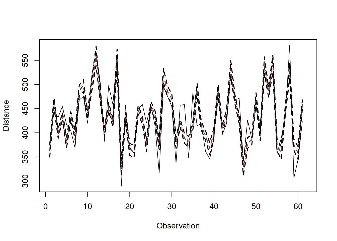
Figure 12.6: Fitted values and confidence interval for the stopping distance model.
The same fitted values and interval can be presented differently on the actuals vs fitted plot:
plot(fitted(slmSpeedDistance),actuals(slmSpeedDistance),
     xlab="Fitted",ylab="Actuals")
abline(a=0,b=1,col="darkblue",lwd=2)
lines(sort(fitted(slmSpeedDistance)),
      slmSpeedDistanceCI$lower[order(fitted(slmSpeedDistance))],
      col="darkred", lwd=2)
lines(sort(fitted(slmSpeedDistance)),
      slmSpeedDistanceCI$upper[order(fitted(slmSpeedDistance))],
      col="darkred", lwd=2)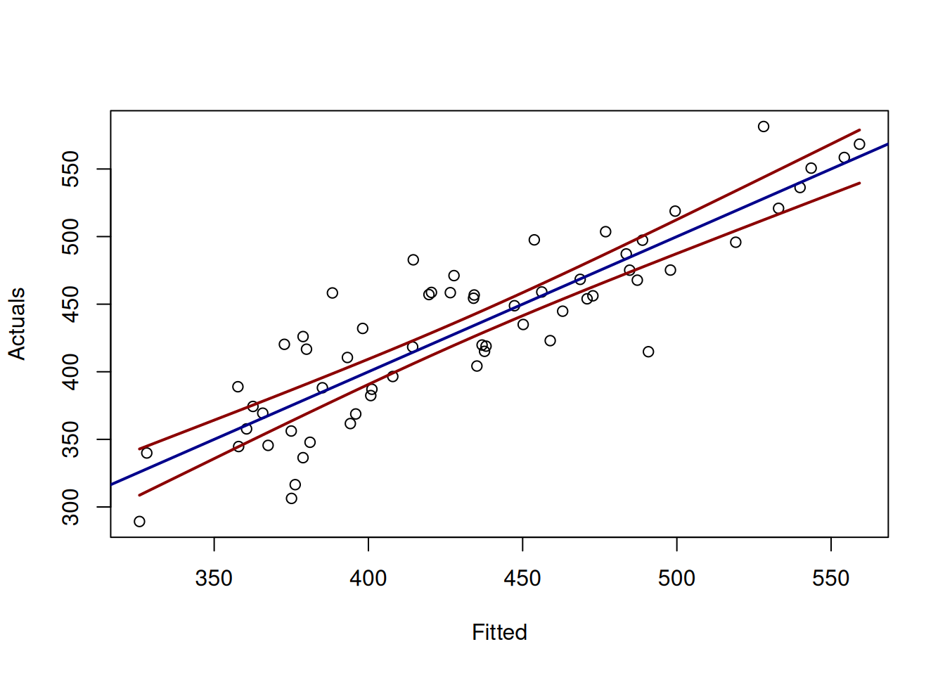
Figure 12.7: Actuals vs Fitted and confidence interval for the stopping distance model.
Figure 12.7 demonstrates the actuals vs fitted plot, together with the 95% confidence interval around the line, demonstrating where the line would be expected to be in 95% of the cases if we re-estimate the model many times. We also see that the uncertainty of the regression line is lower in the middle of the data, but expands in the tails. Conceptually, this happens because the regression line, estimated via OLS, always passes through the average point of the data \((\bar{x},\bar{y})\) and the variability in this point is lower than the variability in the tails.
If we are not interested in the uncertainty of the regression line, but rather in the uncertainty of the observations, we can refer to prediction interval. The variance in this case is: \[\begin{equation} \mathrm{V}(y_j| \mathbf{x}_j) = \mathrm{V}(b_0 + b_1 x_{1,j} + b_2 x_{2,j} + \dots + b_{k-1} x_{k-1,j} + e_j) , \tag{12.9} \end{equation}\] which can be simplified to (if assumptions of regression model hold, see Section 15): \[\begin{equation} \mathrm{V}(y_j| \mathbf{x}_j) = \mathrm{V}(\hat{y}_j| \mathbf{x}_j) + \hat{\sigma}^2, \tag{12.10} \end{equation}\] where \(\hat{\sigma}^2\) is the variance of the residuals \(e_j\). As we see from the formula (12.10), the variance in this case is larger than (12.7), which will result in wider interval than the confidence one. We can use normal distribution for the construction of the interval in this case (using formula similar to (12.8)), as long as we can assume that \(\epsilon_j \sim \mathcal{N}(0,\sigma^2)\).
In R, this can be done via the very same predict() function with interval="prediction":
Based on this, we can construct graphs similar to 12.6 and 12.7.
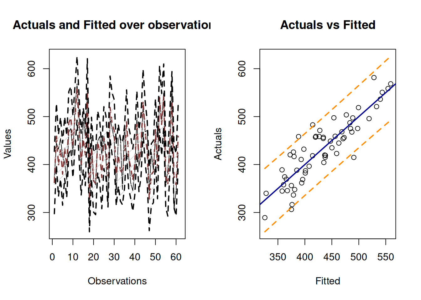
Figure 12.8: Fitted values and prediction interval for the stopping distance model.
Figure 12.8 shows the prediction interval for values over observations and for actuals vs fitted. As we see, the interval is wider in this case, covering only 95% of observations (there are 2 observations outside it).
In forecasting, prediction interval has a bigger importance than the confidence interval. This is because we are typically interested in capturing the uncertainty about the observations, not about the estimate of a line. Typically, the prediction interval would be constructed for some holdout data, which we did not have at the model estimation phase. In the example with stopping distance, we could see what would happen if the speed of a car was, for example, 30mph:
slmSpeedDistanceForecast <- predict(slmSpeedDistance,newdata=data.frame(speed=30),
                                    interval="prediction")
plot(slmSpeedDistanceForecast)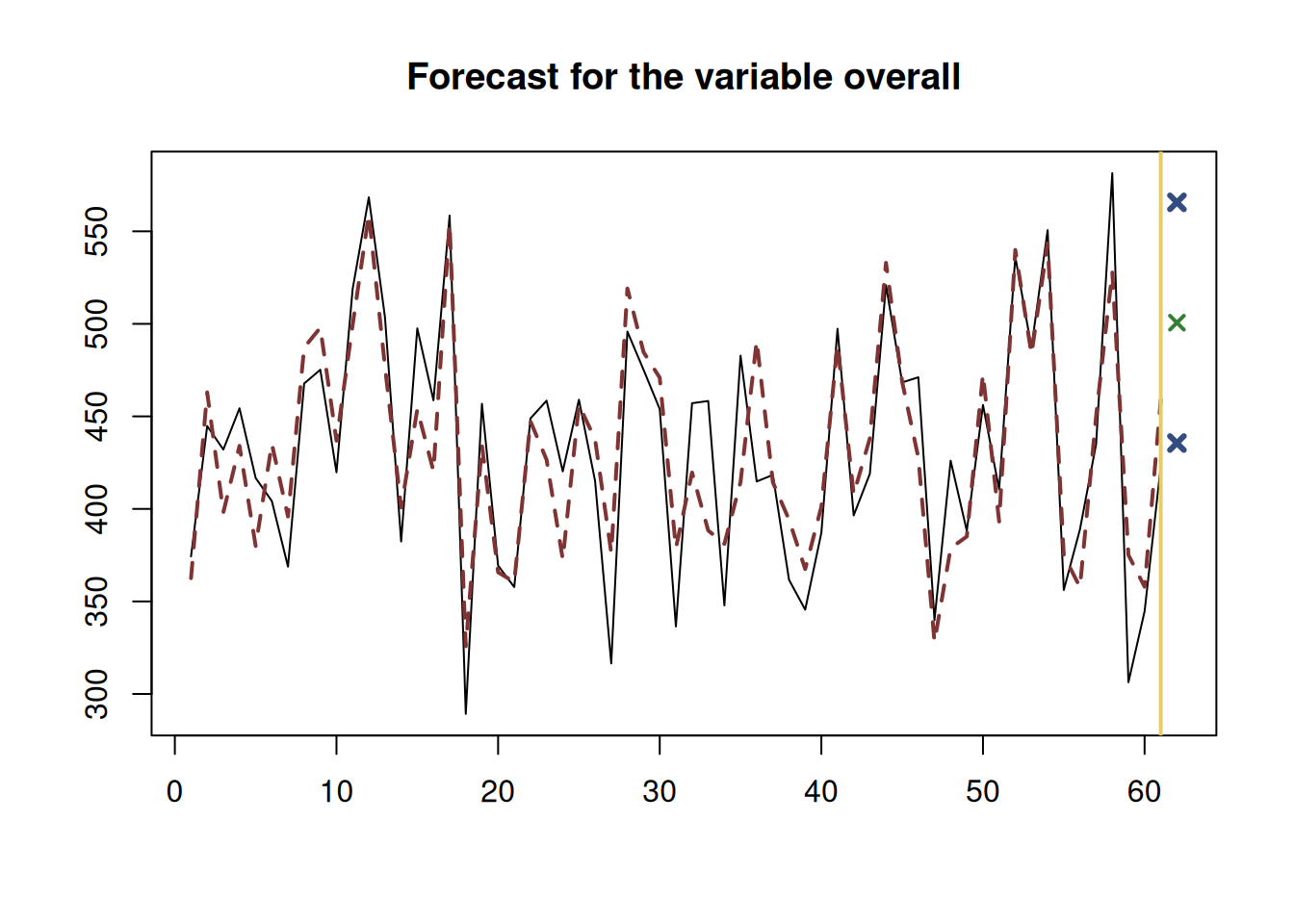
Figure 12.9: Forecast of the stopping distance for the speed of 30mph.
Figure 12.9 shows the point forecast (the expected stopping distance if the speed of car was 30mph) and the 95% prediction interval (we expect that in 95% of the cases, the cars will have the stopping distance between 66.865 and 133.921 feet.