Chapter 12 Uncertainty in regression
Coming back to the example of mileage vs weight of cars, the estimated simple linear regression on the data was mpg=37.29-5.34wt+et. But what would happen if we estimate the same model on a different sample of data (e.g. 15 first observations instead of 32)?
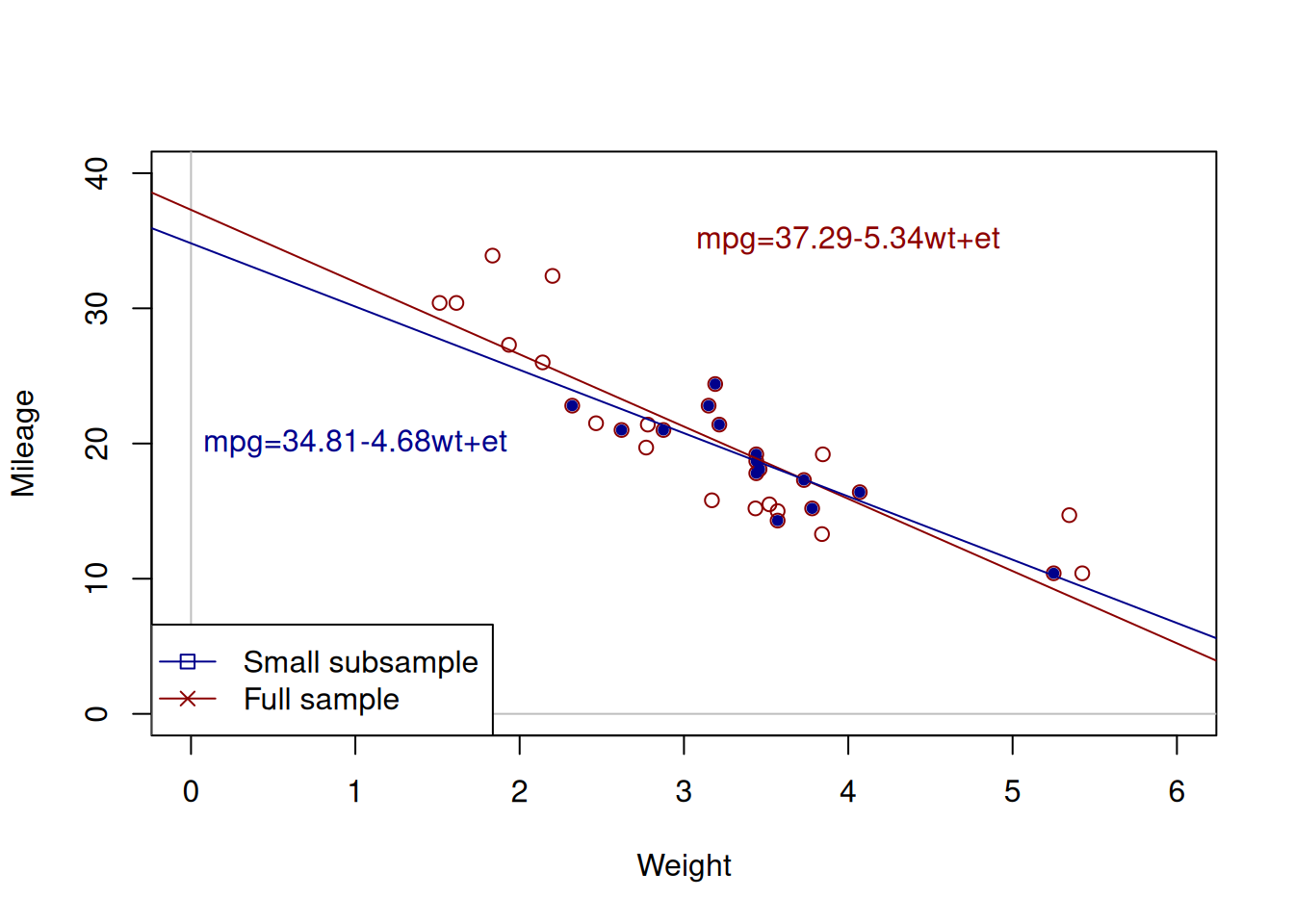
Figure 12.1: Weight vs mileage and two regression lines.
Figure 12.1 shows the two lines: the red one corresponds to the larger sample, while the blue one corresponds to the small one. We can see that these lines have different intercepts and slope parameters. So, which one of them is correct? An amateur analyst would say that the one that has more observations is the correct model. But a more experienced statistician would tell you that none of the two is correct. They are both estimated on a sample of data and they both inevitably inherit the uncertainty of the data, making them both incorrect if we compare them to the hypothetical true model. This means that whatever regression model we estimate on a sample of data, it will be incorrect as well.
This uncertainty about the regression line actually comes to the uncertainty of estimates of parameters of the model. In order to see it more clearly, consider the example with Speed and Stopping Distances of Cars dataset from datasets package (?cars):
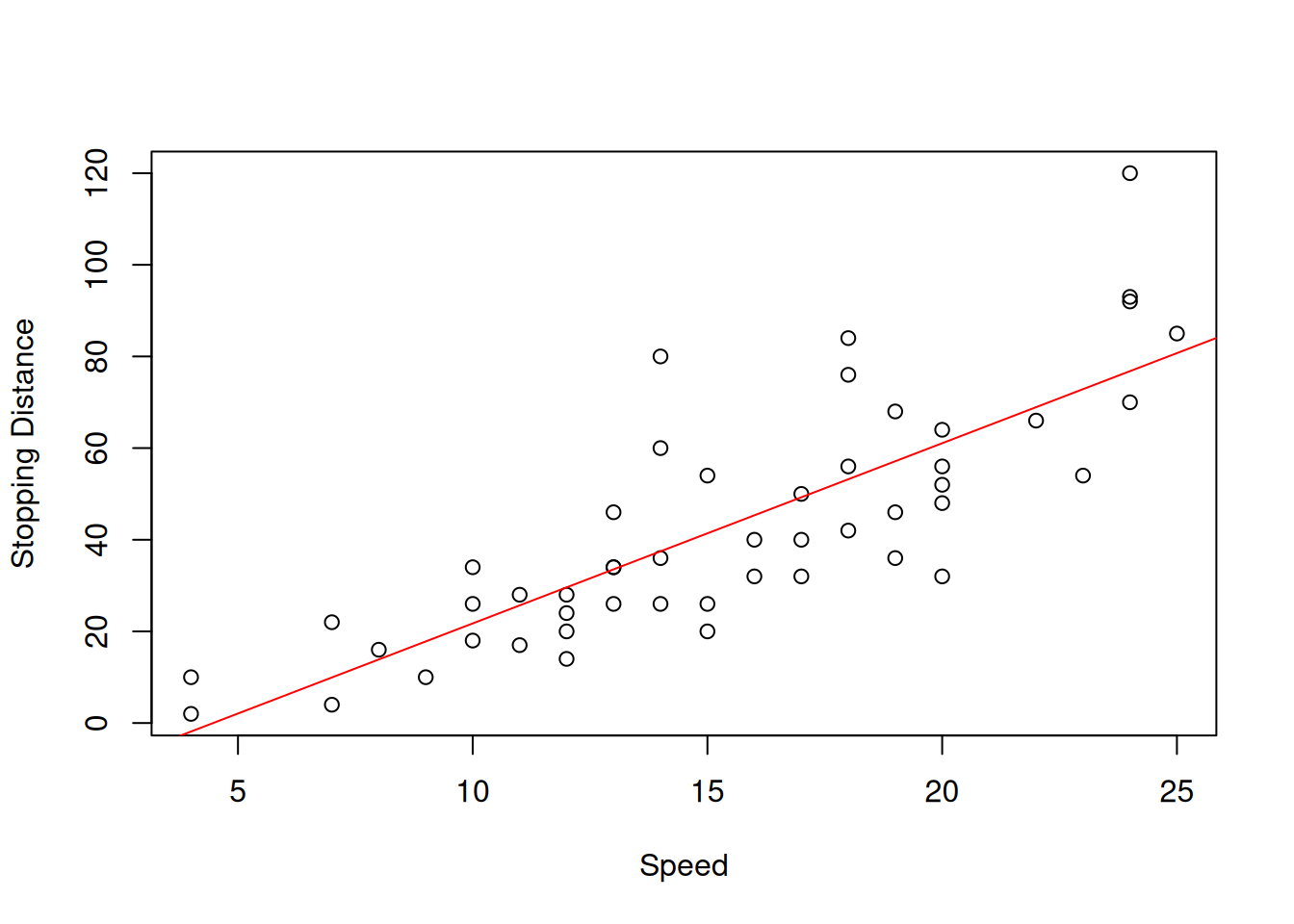
Figure 12.2: Speed vs stopping distance of cars
While the linear relation between these variables might be not the the most appropriate, it suffices for demonstration purposes. What we will do for this example is fit the model and then use a simple bootstrap technique to get estimates of parameters of the model. We will do that using coefbootstrap() method from greybox package. The bootstrap technique implemented in the function applies the same model to subsamples of the original data and returns a matrix with parameters. This way we get an idea about the empirical uncertainty of parameters:
Based on that we can plot the histograms of the estimates of parameters.
par(mfcol=c(1,2))
hist(slmSpeedDistanceBootstrap$coefficients[,1],
     xlab="Intercept", main="")
hist(slmSpeedDistanceBootstrap$coefficients[,2],
     xlab="Slope", main="")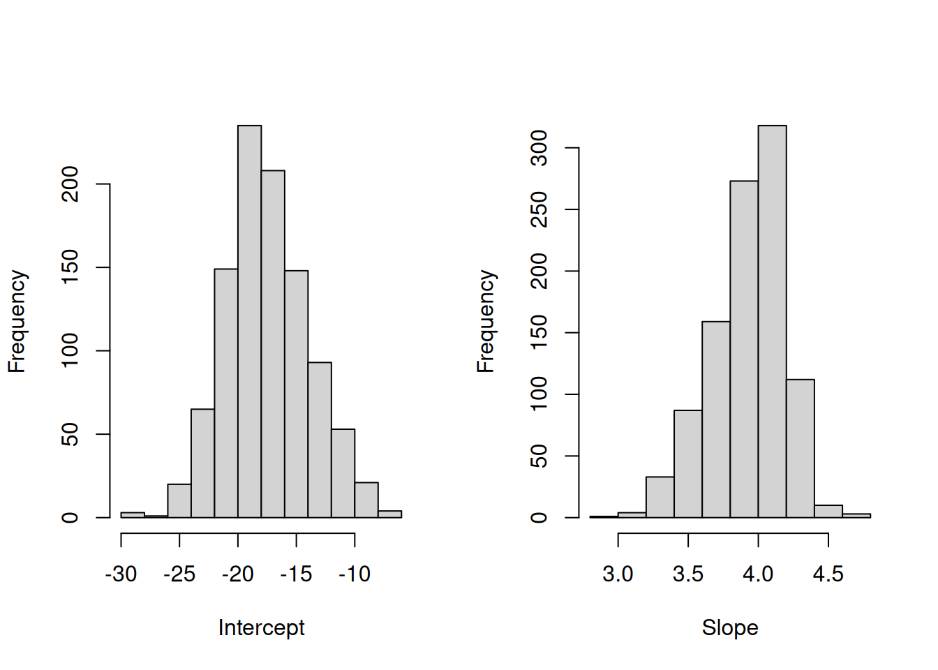
Figure 12.3: Distribution of bootstrapped parameters of a regression model
Figure 12.3 shows the uncertainty around the estimates of parameters. These distributions look similar to the normal distribution. In fact, if we repeated this example thousands of times, the distribution of estimates of parameters would indeed follow the normal one due to CLT (if the assumptions hold, see Sections 6.2 and 15). As a result, when we work with regression we should take this uncertainty about the parameters into account. This applies to both parameters analysis and forecasting.