4.10 Gamma distribution
Finally, another distribution that will be useful for ETS and ARIMA is Gamma (\(\mathcal{\Gamma}\)), which is parameterised using shape \(\xi\) and scale \(s\), and is defined for positive values only. This distribution is useful because it is scalable and is as flexible as (\(\mathcal{IG}\)) in terms of possible shapes. It also has an important scalability property (simila to \(\mathcal{IG}\)), but the shape needs to be restricted in order to make sense in ETS model: \[\begin{equation} \text{if } (1+\epsilon_t) \sim \mathcal{\Gamma}(s^{-1}, s) \text{, then } y_t = \mu_{y,t} \times (1+\epsilon_t) \sim \mathcal{\Gamma}\left(s^{-1}, s \mu_{y,t} \right), \tag{4.26} \end{equation}\] implying that the scale of the model changes together with the expectation. The restriction on the shape parameters is needed in order to make the expectation of \((1+\epsilon_t)\) equal to one. The PDF of the distribution of \(1+\epsilon_t\) is:
\[\begin{equation} f(1+\epsilon_t) = \frac{1}{\Gamma(s^{-1}) (s)^{s^{-1}}} (1+\epsilon_t)^{s^{-1}-1}\exp \left(-\frac{1+\epsilon_t}{s}\right) . \tag{4.27} \end{equation}\] However, the scale \(s\) cannot be estimated via the maximisation of likelihood analytically due to the restriction (4.26). Luckliy, the method of moments can be used instead, where based on the expectation and variance we get: \[\begin{equation} \hat{s} = \frac{1}{T} \sum_{t=1}^T e_t^2 , \tag{4.28} \end{equation}\] where \(e_t\) is the estimate of \(\epsilon_t\). So, imposing the restrictions (4.26) implies that the scale of \(\mathcal{\Gamma}\) is equal to the variance of the error term.
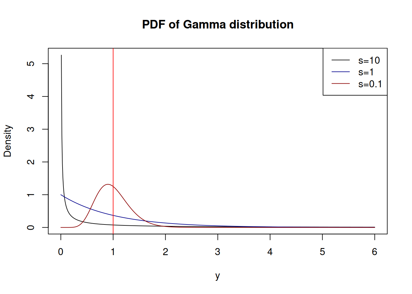
Figure 4.14 demonstrates how the PDF of \(\mathcal{\Gamma}(s^{-1},s)\) looks for different values of \(s\):

Figure 4.14: Probability Density Functions of Gamma distribution
With the increase of the shape \(\xi=s^{-1}\) (in our case this implies the decrease of variance \(s\)), \(\mathcal{\Gamma}\) distribution converges to the normal one with \(\mu=\xi s=1\) and variance \(\sigma^2=s\). This demonstrates indirectly that the estimate of the scale (4.28) maximises the likelihood of the function (4.27), although I do not have any proper proof of this.