4.4 Laplace distribution
A more exotic distribution is Laplace, which has some similarities with Normal, but has higher excess. It has the following PDF:
\[\begin{equation} f(y_t) = \frac{1}{2 s} \exp \left( -\frac{\left| y_t - \mu_{y,t} \right|}{s} \right) , \tag{4.9} \end{equation}\] where \(s\) is the scale parameter, which, when estimated using likelihood, is equal to the Mean Absolute Error (MAE): \[\begin{equation} \hat{s} = \frac{1}{T} \sum_{t=1}^T \left| y_t - \hat{\mu}_{y,t} \right| . \tag{4.10} \end{equation}\]
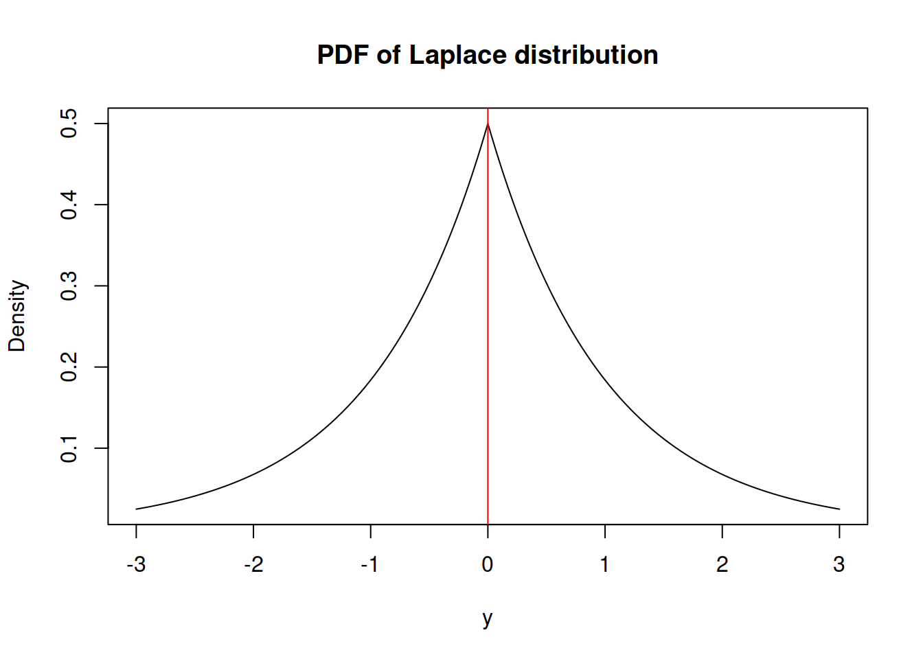
It has the shape shown on Figure 4.9.

Figure 4.9: Probability Density Function of Laplace distribution
Similar to the Normal distribution, the skewness of Laplace is equal to zero. However, it has fatter tails - its kurtosis is equal to 6 instead of 3.
The variance of the random variable following Laplace distribution is equal to: \[\begin{equation} \sigma^2 = 2 s^2. \tag{4.11} \end{equation}\]
The dlaplace, qlaplace, plaplace and rlaplace functions from greybox package implement different sides of Laplace distribution in R.