4.9 Inverse Gaussian distribution
An exotic distribution that will be useful for what comes in this textbook is the Inverse Gaussian (\(\mathcal{IG}\)), which is parameterised using mean value \(\mu_{y,t}\) and either the dispersion parameter \(s\) or the scale \(\lambda\) and is defined for positive values only. This distribution is useful because it is scalable and has some similarities with the Normal one. In our case, the important property is the following: \[\begin{equation} \text{if } (1+\epsilon_t) \sim \mathcal{IG}(1, s) \text{, then } y_t = \mu_{y,t} \times (1+\epsilon_t) \sim \mathcal{IG}\left(\mu_{y,t}, \frac{s}{\mu_{y,t}} \right), \tag{4.23} \end{equation}\] implying that the dispersion of the model changes together with the expectation. The PDF of the distribution of \(1+\epsilon_t\) is:
\[\begin{equation} f(1+\epsilon_t) = \frac{1}{\sqrt{2 \pi s (1+\epsilon_t)^3}} \exp \left( -\frac{\epsilon_t^2}{2 s (1+\epsilon_t)} \right) , \tag{4.24} \end{equation}\] where the dispersion parameter can be estimated via maximising the likelihood and is calculated using: \[\begin{equation} \hat{s} = \frac{1}{T} \sum_{t=1}^T \frac{e_t^2}{1+e_t} , \tag{4.25} \end{equation}\] where \(e_t\) is the estimate of \(\epsilon_t\). This distribution becomes very useful for multiplicative models, where it is expected that the data can only be positive.
Figure 4.13 shows how the PDF of \(\mathcal{IG}(1,s)\) looks for different values of the dispersion \(s\)
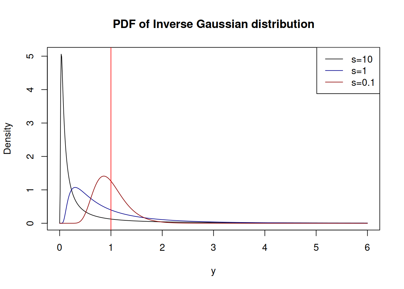
Figure 4.13: Probability Density Functions of Inverse Gaussian distribution
statmod package implements density, quantile, cumulative and random number generator functions for the \(\mathcal{IG}\).