This book is in Open Review. I want your feedback to make the book better for you and other readers. To add your annotation, select some text and then click the on the pop-up menu. To see the annotations of others, click the button in the upper right hand corner of the page

4.5 S distribution

This is something relatively new, but not ground braking. I have derived S distribution few years ago, but have never written a paper on that. It has the following density function (it is as a special case of Generalised Normal distribution, when \(\beta=0.5\)): \[\begin{equation} f(y_t) = \frac{1}{4 s^2} \exp \left( -\frac{\sqrt{|y_t - \mu_{y,t}|}}{s} \right) , \tag{4.12} \end{equation}\] where \(s\) is the scale parameter. If estimated via maximum likelihood, the scale parameter is equal to: \[\begin{equation} \hat{s} = \frac{1}{2T} \sum_{t=1}^T \sqrt{\left| y_t - \hat{\mu}_{y,t} \right|} , \tag{4.13} \end{equation}\] which corresponds to the minimisation of a half of “Mean Root Absolute Error” or “Half Absolute Moment” (HAM). This is a more exotic type of scale, but the main benefit of this distribution is sever heavy tails - it has kurtosis of 25.2. It might be useful in cases of randomly occurring incidents and extreme values (Black Swans?).

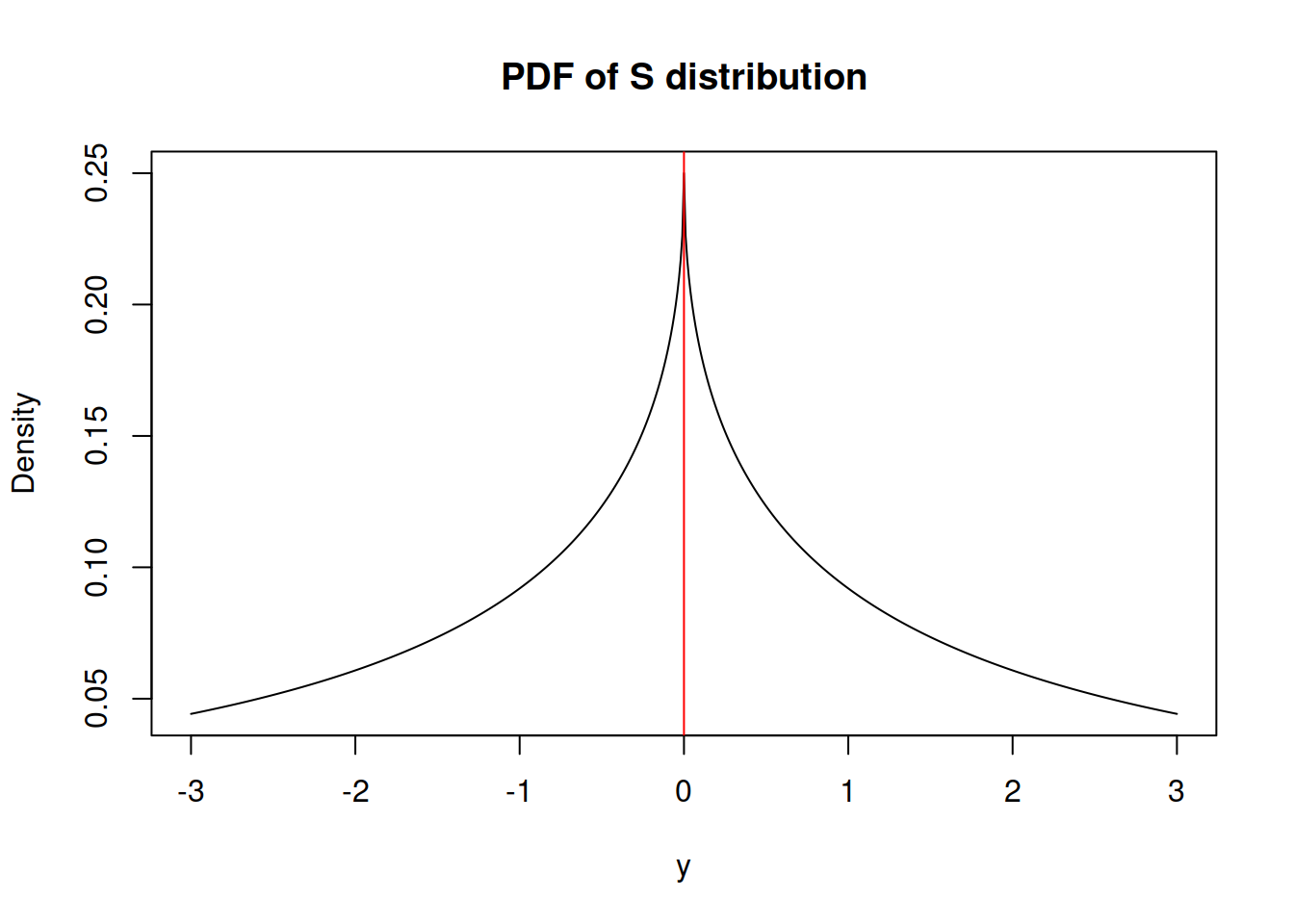
Figure 4.10: Probability Density Function of S distribution

The variance of the random variable following S distribution is equal to: \[\begin{equation} \sigma^2 = 120 s^4. \tag{4.14} \end{equation}\]

The ds, qs, ps and rs from greybox package implement the density, quantile, cumulative and random generation functions.