4.7 Asymmetric Laplace distribution
Asymmetric Laplace distribution (\(\mathcal{AL}\)) can be considered as a two Laplace distributions with different parameters \(s\) for left and right sides from the location \(\mu_{y,t}\). There are several ways to summarise the probability density function, the neater one relies on the asymmetry parameter \(\alpha\) (Yu and Zhang, 2005): \[\begin{equation} f(y_t) = \frac{\alpha (1- \alpha)}{s} \exp \left( -\frac{y_t - \mu_{y,t}}{s} (\alpha - I(y_t \leq \mu_{y,t})) \right) , \tag{4.18} \end{equation}\] where \(s\) is the scale parameter, \(\alpha\) is the skewness parameter and \(I(y_t \leq \mu_{y,t})\) is the indicator function, which is equal to one, when the condition is satisfied and to zero otherwise. The scale parameter \(s\) estimated using likelihood is equal to the quantile loss: \[\begin{equation} \hat{s} = \frac{1}{T} \sum_{t=1}^T \left(y_t - \hat{\mu}_{y,t} \right)(\alpha - I(y_t \leq \hat{\mu}_{y,t})) . \tag{4.19} \end{equation}\] Thus maximising the likelihood (4.18) is equivalent to estimating the model via the minimisation of \(\alpha\) quantile, making this equivalent to quantile regression approach. So quantile regression models assume indirectly that the error term in the model is \(\epsilon_t \sim \mathcal{AL}(0, s, \alpha)\) (Geraci and Bottai, 2007).
Depending on the value of \(\alpha\), the distribution can have different shapes, shown in Figure 4.12.
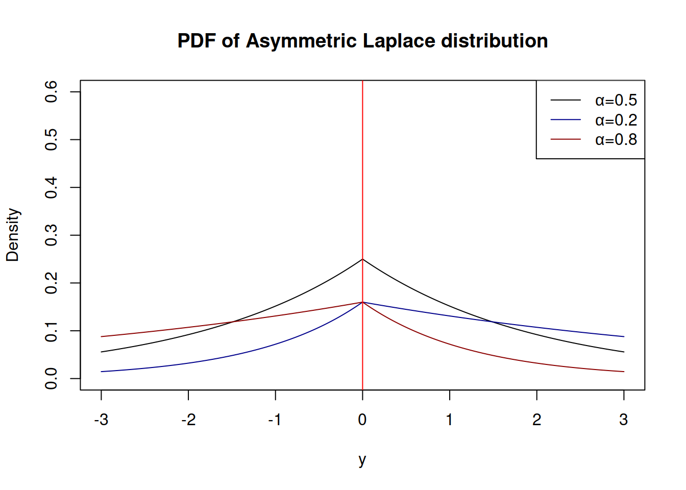
Figure 4.12: Probability Density Functions of Asymmetric Laplace distribution
Similarly to \(\mathcal{GN}\) distribution, the parameter \(\alpha\) can be estimated during the maximisation of the likelihood, although it makes more sense to set it to some specific values in order to obtain the desired quantile of distribution.
The variance of the random variable following Asymmetric Laplace distribution is equal to: \[\begin{equation} \sigma^2 = s^2\frac{(1-\alpha)^2+\alpha^2}{\alpha^2(1-\alpha)^2}. \tag{4.20} \end{equation}\]
Functions dalaplace, qalaplace, palaplace and ralaplace from greybox package implement the Asymmetric Laplace distribution.
References
• Geraci, M., Bottai, M., 2007. Quantile regression for longitudinal data using the asymmetric Laplace distribution. Biostatistics. 8, 140–154. https://doi.org/10.1093/biostatistics/kxj039
• Yu, K., Zhang, J., 2005. A three-parameter asymmetric laplace distribution and its extension. Communications in Statistics - Theory and Methods. 34, 1867–1879. https://doi.org/10.1080/03610920500199018