4.6 Generalised Normal distribution
Generalised Normal (\(\mathcal{GN}\)) distribution (as the name says) is a generalisation for Normal distribution, which also includes Laplace and S as special cases (Nadarajah, 2005). There are two versions of this distribution: one with a shape and another with a skewness parameter. We are mainly interested in the first one, which has the following PDF: \[\begin{equation} f(y_t) = \frac{\beta}{2 s \Gamma(\beta^{-1})} \exp \left( -\left(\frac{|y_t - \mu_{y,t}|}{s}\right)^{\beta} \right), \tag{4.15} \end{equation}\] where \(\beta\) is the shape parameter, and \(s\) is the scale of the distribution, which, when estimated via MLE, is equal to: \[\begin{equation} \hat{s} = \sqrt[^{\beta}]{\frac{\beta}{T} \sum_{t=1}^T\left| y_t - \hat{\mu}_{y,t} \right|^{\beta}}, \tag{4.16} \end{equation}\] which has MSE, MAE and HAM as special cases, when \(\beta\) is equal to 2, 1 and 0.5 respectively. The parameter \(\beta\) influences the kurtosis directly, it can be calculated for each special case as \(\frac{\Gamma(5/\beta)\Gamma(1/\beta)}{\Gamma(3/\beta)^2}\). The higher \(\beta\) is, the lower the kurtosis is.
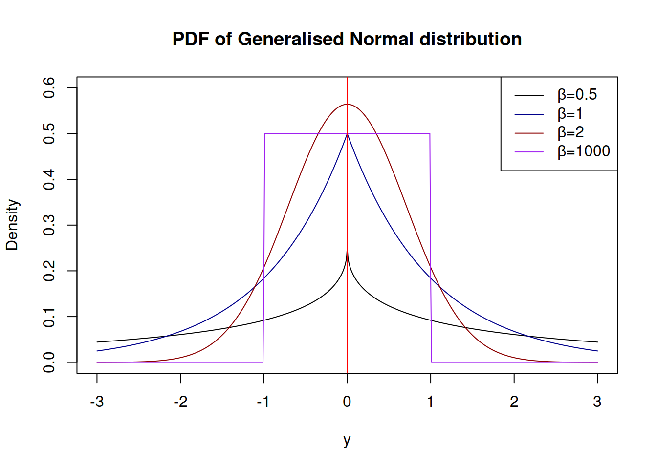
The advantage of \(\mathcal{GN}\) distribution is its flexibility. In theory, it is possible to model extremely rare events with this distribution, if the shape parameter \(\beta\) is fractional and close to zero. Alternatively, when \(\beta \rightarrow \infty\), the distribution converges point-wise to the uniform distribution on \((\mu_{y,t} - s, \mu_{y,t} + s)\).
Note that the estimation of \(\beta\) is a difficult task, especially, when it is less than 2 - the MLE of it looses properties of consistency and asymptotic normality.
Depending on the value of \(\beta\), the distribution can have different shapes shown in Figure 4.11

Figure 4.11: Probability Density Functions of Generalised Normal distribution
Typically, estimating \(\beta\) consistently is a tricky thing to do, especially if it is less than one. Still, it is possible to do that by maximising the likelihood function (4.15).
The variance of the random variable following Generalised Normal distribution is equal to: \[\begin{equation} \sigma^2 = s^2\frac{\Gamma(3/\beta)}{\Gamma(1/\beta)}. \tag{4.17} \end{equation}\]
The working functions for the Generalised Normal distribution are implemented in the greybox package for R.
References
• Nadarajah, S., 2005. A generalized normal distribution. Journal of Applied Statistics. 32, 685–694. https://doi.org/10.1080/02664760500079464